2-Dimensional Motion

Kseniia Suleimanova Fall 2025

The Main Idea

When objects move in 2-dimensional space, their motion can be described in [math]\displaystyle{ \hat{x},\ \hat{y} }[/math] coordinates. The motion for each of those axes can be viewed independently. Another approach is using vectors (i.e. coordinate (5, 3) can be seen as vector [math]\displaystyle{ \langle 5,\ 3 \rangle }[/math]).

Displacement and distance

Imagine we have 2 points and origin O: A = [math]\displaystyle{ \langle a,\ b \rangle }[/math], B = [math]\displaystyle{ \langle c,\ d \rangle }[/math]

A point particle moves from origin to point A and then to point B. The displacement can be viewed as adding those vectors: [math]\displaystyle{ \langle a,\ b \rangle + \langle c,\ d \rangle = \langle a + c,\ b + d \rangle }[/math].

The distance is the sum of magnitudes of those vectors: [math]\displaystyle{ \sqrt{a^{2} + b^{2}} + \sqrt{c^{2} + d^{2}} }[/math]

Moving with a constant velocity

Velocity is the derivative of the position vector. In 2-dimensional space velocity looks the following: [math]\displaystyle{ \vec{v} = \frac{\Delta \vec{r}}{\Delta t} = \left\langle \frac{\Delta x}{\Delta t},\frac{\Delta y}{\Delta t} \right\rangle }[/math], so moving for [math]\displaystyle{ t }[/math] seconds with velocity [math]\displaystyle{ \vec{r} }[/math] can be represented as [math]\displaystyle{ \vec{v} \cdot t = \left\langle \frac{\Delta x}{\Delta t} \cdot t,\frac{\Delta y}{\Delta t} \cdot t \right\rangle }[/math]

Moving with constant acceleration

In 2-dimensional space acceleration is [math]\displaystyle{ \vec{a} = \frac{\Delta \vec{v}}{\Delta t}= \left\langle \frac{\Delta v_x}{\Delta t},\frac{\Delta v_y}{\Delta t} \right\rangle }[/math].

A standard formula for position update is still applicable for vectors in 2-dimensional space: [math]\displaystyle{ \vec{r}(t)=\vec{r}_0+\vec{v}_0 t+\tfrac{1}{2}\vec{a}\,t^{2}=\langle x_0+v_{0x}t+\tfrac{1}{2}a_x t^{2},\ y_0+v_{0y}t+\tfrac{1}{2}a_y t^{2}\rangle }[/math]

Computational models

Projectile motion

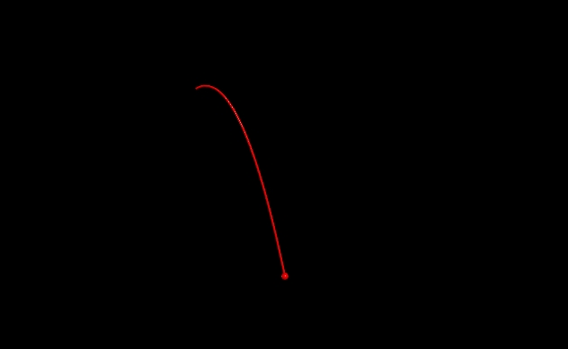
https://www.glowscript.org/#/user/ksuleimanova/folder/MyPrograms/program/projectilemotiondemo - link to execute the code

Web VPython 3.2

scene.range = 10
scene.center = vector(5, 5, 0)
r = vector(0, 10, 0)
v = vector(3, 2, 0)
a = vector(0, -9.8, 0)

dt = 0.05

ball = sphere(pos=r, radius=0.2, color=color.red, make_trail=True)

gx = graph(title="Projectile Motion",
           xtitle="Time, s", ytitle="Position, m")

xplot = gcurve(color=color.blue, label="x(t)")
yplot = gcurve(color=color.green, label="y(t)")

t = 0

while r.y >= 0:
    rate(100)
    v = v + a * dt
    r = r + v * dt
    ball.pos = r
    xplot.plot(t, r.x)
    yplot.plot(t, r.y)
    t = t + dt

In this code the position is updated every small increment of time, using the position update formula for constant acceleration, involving velocity first, and then position:

v = v + a * dt
r = r + v * dt

Circular motion

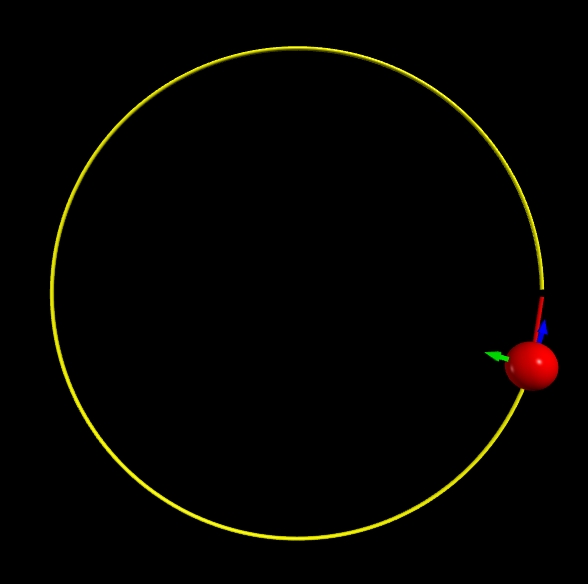
In the circular velocity magnitude is constant, while its direction changes.

https://www.glowscript.org/#/user/ksuleimanova/folder/MyPrograms/program/circularmotion - link to execute the code

Web VPython 3.2


scene.width = 600
scene.height = 600
R = 5
omega = 1
dt = 0.05

particle = sphere(pos=vector(R,0,0), radius=0.5, color=color.red, make_trail=True)
arrow_velocity = arrow(pos=particle.pos, axis=vector(0,1,0), color=color.blue, shaftwidth=0.1)
arrow_accel = arrow(pos=particle.pos, axis=vector(0,1,0), color=color.green, shaftwidth=0.1)

t = 0

v_mag = 3
velocity = vector(0, v_mag, 0)
path = curve(color=color.yellow)

while t < 10:
    particle.pos = particle.pos + velocity*dt
    accel = - (velocity.mag**2 / R) * particle.pos.norm()
    velocity = velocity + accel*dt
    arrow_velocity.pos = particle.pos
    arrow_velocity.axis = velocity.norm()
    arrow_accel.pos = particle.pos
    arrow_accel.axis = accel.norm()
    path.append(pos=particle.pos)
    t += dt

This code also uses position update for each time increment.

Examples

Easy

Problem: A point particle starts at a point (0, 5)m on a flat surface an moves with a constant velocity [math]\displaystyle{ \langle 4,\ 1 \rangle m }[/math]. Find it's position after 5 seconds.

Solution: Intial position vector is [math]\displaystyle{ \langle 0,\ 5 \rangle m }[/math] As the velocity is constant, acceleration is 0. Insert all the data into the position update formula: [math]\displaystyle{ \vec{r}(t)=\vec{r}_0+\vec{v}_0 t+\tfrac{1}{2}\vec{a}\,t^{2}=\vec{r}_0+\vec{v}_0 t + 0 = \langle 0,\ 5 \rangle + \langle 4,\ 1 \rangle \cdot 5 = \langle 20,\ 10 \rangle m }[/math]

Medium

Problem: A bug on the table travels from point (1, 2)m to point (2, 1)m and then to (2, 2)m. The whole path takes 2 seconds. Find average speed and average velocity.

Solution: Displacement is [math]\displaystyle{ \langle 2,\ 2 \rangle - \langle 1,\ 2 \rangle = \langle 1,\ 0 \rangle m }[/math] Distance is the length of the path: [math]\displaystyle{ \sqrt{(2 - 1)^{2} + (1 - 2)^{2}} + \sqrt{(2 - 2)^{2} + (2 - 1)^{2}} = \sqrt{2} + \sqrt{1} = 2.41 m }[/math]

Average speed: [math]\displaystyle{ 2.41 / 2 = 1.21 m/s }[/math]

Average velocity: [math]\displaystyle{ \langle 1,\ 0 \rangle / 2 = \langle 0.5,\ 0 \rangle m/s }[/math]

Hard

Problem: The ball is thrown from the building with the height 10 meters. The initial velocity of the ball is [math]\displaystyle{ \langle 3,\ 2 \rangle \textit{m/s} }[/math] find the time and position when the ball reaches its maximum height.

Solution: This is the projectile motion problem in 2-dimensional space. The most convenient approach is to view vertical and horizontal motion independently. We know that horizontal component of the velocity stays the same, while [math]\displaystyle{ \vec{v}_{y} = \vec{v}_{y_{init}} - g t }[/math] - the ball moves with a constant acceleration. For the [math]\displaystyle{ \hat{y} }[/math] we can use the position update formula for constant acceleration [math]\displaystyle{ -g }[/math]: [math]\displaystyle{ r_{y}(t)=r_{y_0}+\vec{v_{y_0}} t-\tfrac{1}{2}\vec{g}\,t^{2} }[/math]. This is a parabola that has a maximum value. Insert numerical values and solve the equation: [math]\displaystyle{ r_{y}(t)=10+2 t-\tfrac{1}{2}\cdot 9.8 \cdot t^{2} }[/math]. Maximum value is achieved at [math]\displaystyle{ t = 0.21 s }[/math]. At [math]\displaystyle{ t_{max} = 0.21 s }[/math] x-coordinate is [math]\displaystyle{ r_{x_{init}} = \vec{v_x} \cdot t_{max} = 0 + 3 \cdot 0.21 = 0.63 m }[/math] y-coordinate is [math]\displaystyle{ r_{y}(0.21)=r_{y_0}+\vec{v_{y_0}} \cdot 0.21-\tfrac{1}{2}\vec{g} \cdot 0.21^{2} = 10 + 3 \cdot 0.21 - \tfrac{1}{2} \cdot 9.8 \cdot 0.21 = 10.41 m }[/math]

Links To Other Topics

• 2-dimensional motion relies on vectors most of the time
• Most projectile motion problems are 2-dimensional
• Centripital motion problems are 2-dimensional as well

See Also

https://youtu.be/w3BhzYI6zXU?si=oivAjOifOPBi_5D4 - vectors and 2D motion

https://youtu.be/On5DpeGQ89I?si=7zqYvWx73W3HYwjG - 2D motion problems with solutions

References

https://ocw.mit.edu/courses/8-01sc-classical-mechanics-fall-2016/pages/week-1-kinematics/3-1-coordinate-system-and-position-vector-in-2d/

https://ocw.mit.edu/courses/8-01sc-classical-mechanics-fall-2016/pages/week-1-kinematics/3-4-projectile-motion/