Integration Techniques for Magnetic Field: Difference between revisions
Rmanathkar3 (talk | contribs) (Created page with "In the study of magnetic fields, many formulas for the magnetic field of different objects are derived by integrating the magnetic field of a small portion of the object over...") |
Rmanathkar3 (talk | contribs) |
||
| (17 intermediate revisions by the same user not shown) | |||
| Line 6: | Line 6: | ||
===Mathematical Model=== | ===Mathematical Model=== | ||
[[File:Biot.png]] and then [[File:BiotR.jpg]] | [[File:Biot.png]] and then [[File:BiotR.jpg]] | ||
===Computational Model=== | |||
This is code from a previous lab that simulates a moving proton creating a magnetic field. Because current creates magnetic field and current is essentially a moving charge, this model helps you to see that the location of the moving charge in relation to the observation location changes the magnitude of the magnetic field. As a result, it is important to consider all the points of a wire and thus all the different locations of a moving charge when finding the net magnetic field of a wire. For this reason, we use integration to find net magnetic field. | |||
from __future__ import division | |||
from visual import * | |||
## Constants | |||
oofpez = 1e-7 | |||
qproton = (-1.6e-19) | |||
## Objects | |||
#Change the initial vector position of the proton below: | |||
proton = sphere(pos=vector(3e-10,0,0), radius=1e-11, color=color.red) | |||
#Change the observation location (position of the tail of the arrow) below: | |||
#Add more arrows to find magnetic field at other observation locations. | |||
#Set axis to (0,0,0) initially and update it in the loop. | |||
barrow1=arrow(pos=vector(0,8e-11,0), axis=vector(0,0,0), color=color.cyan) | |||
barrow2=arrow(pos=vector(0,-8e-11,0), axis=vector(0,0,0), color=color.cyan) | |||
barrow3=arrow(pos=vector(0,0,8e-11), axis=vector(0,0,0), color=color.cyan) | |||
barrow4=arrow(pos=vector(0,0,-8e-11), axis=vector(0,0,0), color=color.cyan) | |||
## Initial values | |||
velocity = vector(-5.2e4,0,0) # Enter the proton's velocity | |||
deltat = 1e-17 # Adjust if program runs too slowly or too quickly | |||
scene.autoscale=0 #Turns off autoscaling. Set to 1 to turn it back on. | |||
## Loop | |||
while proton.x<5e-10: | |||
rate(100) | |||
# For each magnetic field vector: | |||
# 1. Calculate r and rhat | |||
r1 = barrow1.pos - proton.pos | |||
r2 = barrow2.pos - proton.pos | |||
r3 = barrow3.pos - proton.pos | |||
r4 = barrow4.pos - proton.pos | |||
r1hat = norm(r1) | |||
r2hat = norm(r2) | |||
r3hat = norm(r3) | |||
r4hat = norm(r4) | |||
r1mag = mag(r1) | |||
r2mag = mag(r2) | |||
r3mag = mag(r3) | |||
r4mag = mag(r4) | |||
# 2. Calculate the magnetic field vector | |||
B1 = (oofpez)*(qproton)*((cross(velocity,r1hat))/(r1mag**2)) | |||
B2 = (oofpez)*(qproton)*((cross(velocity,r2hat))/(r2mag**2)) | |||
B3 = (oofpez)*(qproton)*((cross(velocity,r3hat))/(r3mag**2)) | |||
B4 = (oofpez)*(qproton)*((cross(velocity,r4hat))/(r4mag**2)) | |||
# 3. Calculate the new axis of the arrow. Scale it appropriately. | |||
barrow1.axis = 5e-9*B1 | |||
barrow2.axis = 5e-9*B2 | |||
barrow3.axis = 5e-9*B3 | |||
barrow4.axis = 5e-9*B4 | |||
# Update the proton's position | |||
proton.pos += velocity * deltat | |||
==Example== | ==Example== | ||
===Simple=== | |||
[[File:ExamplePart1.jpg]] | |||
[[File:ExamplePart2.jpg]] | |||
===Middling=== | |||
[[File:SquareWireProblem.jpg]] | |||
[[File:SquareWireSoln2.jpg]] | |||
[[File:SquareWireSoln1.jpg]] | |||
===Hard=== | |||
[[File:ExampleMiddlingPart1.jpg]] | |||
[[File:ExampleMiddlingPart2.jpg]] | |||
==Connection== | ==Connection== | ||
Calculus was invented to do physics. By integrating over an object to find its magnetic field, you are performing one of the basic operations on which physics is founded on, which is used to derive other formulas. Additionally, using this method should allow you to find the magnetic field of any object, no matter its shape or size. | Calculus was invented to do physics. By integrating over an object to find its magnetic field, you are performing one of the basic operations on which physics is founded on, which is used to derive other formulas. Additionally, using this method should allow you to find the magnetic field of any object, no matter its shape or size. However, calculus as a whole can be applied to a variety of different areas. Integration specifically is essentially used to find the sum of something with infinite parts. For example, I am an industrial engineer, so if given a function of the output of a machine in regards to time, I could use integration to find the total output of the machine, which can help me later on in efficiency calculations. | ||
==History== | |||
Isaac Newton and Gottfried Leibniz are the two men to whom the discovery of calculus is usually attributed to. However, both men thought of calculus in different ways. Newton thought of calculus with the variables x and y changing over time and computed the tangent of curves using finite velocities of these two variables. However, Leibniz thought of calculus in terms of dx and dy being the difference in close, successive values in a sequence. Because Leibniz used more uniform notation when creating calculus, today's calculus symbols and terms are typically based of Leibniz's original work. | |||
Latest revision as of 14:58, 3 December 2015
In the study of magnetic fields, many formulas for the magnetic field of different objects are derived by integrating the magnetic field of a small portion of the object over the entire area of the object. Often times, you will also be expected to derive your own formulas for less common shapes.
The Main Idea
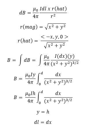
All integration for magnetic fields is based on the Biot-Savart Law for currents, which is ![]() . First, you will take a small portion of the object and call its position Δl. Then find the unit vector from this point to the observation location. Then, take the cross-product of these two vectors and you should end up with a vector that only exists in one dimension (x, y, or z). Now set up your integral by first taking out all the constants from the equation and putting them outside the integral. This should be your mu(naught)/4(pi) and your current. Inside the integral, keep the cross product of the two vectors over r^2, as those are the values that can change during integration. Then set up your limits of integration by going over the full area/length of the object. For example, if you have a rod, integrate over the length of the rod. If you have a loop, integrate from 0 to 2(pi) for the full area of the loop.
. First, you will take a small portion of the object and call its position Δl. Then find the unit vector from this point to the observation location. Then, take the cross-product of these two vectors and you should end up with a vector that only exists in one dimension (x, y, or z). Now set up your integral by first taking out all the constants from the equation and putting them outside the integral. This should be your mu(naught)/4(pi) and your current. Inside the integral, keep the cross product of the two vectors over r^2, as those are the values that can change during integration. Then set up your limits of integration by going over the full area/length of the object. For example, if you have a rod, integrate over the length of the rod. If you have a loop, integrate from 0 to 2(pi) for the full area of the loop.
Mathematical Model
Computational Model
This is code from a previous lab that simulates a moving proton creating a magnetic field. Because current creates magnetic field and current is essentially a moving charge, this model helps you to see that the location of the moving charge in relation to the observation location changes the magnitude of the magnetic field. As a result, it is important to consider all the points of a wire and thus all the different locations of a moving charge when finding the net magnetic field of a wire. For this reason, we use integration to find net magnetic field.
    from __future__ import division
    from visual import *
- Constants
    oofpez = 1e-7
    qproton = (-1.6e-19)
- Objects
- Change the initial vector position of the proton below:
proton = sphere(pos=vector(3e-10,0,0), radius=1e-11, color=color.red)
- Change the observation location (position of the tail of the arrow) below:
- Add more arrows to find magnetic field at other observation locations.
- Set axis to (0,0,0) initially and update it in the loop.
    barrow1=arrow(pos=vector(0,8e-11,0), axis=vector(0,0,0), color=color.cyan)
    barrow2=arrow(pos=vector(0,-8e-11,0), axis=vector(0,0,0), color=color.cyan)
    barrow3=arrow(pos=vector(0,0,8e-11), axis=vector(0,0,0), color=color.cyan)
    barrow4=arrow(pos=vector(0,0,-8e-11), axis=vector(0,0,0), color=color.cyan)
- Initial values
    velocity = vector(-5.2e4,0,0) # Enter the proton's velocity
    deltat = 1e-17 # Adjust if program runs too slowly or too quickly
scene.autoscale=0 #Turns off autoscaling. Set to 1 to turn it back on.
- Loop
while proton.x<5e-10:
   rate(100)
   # For each magnetic field vector:
   # 1. Calculate r and rhat

   r1 =  barrow1.pos - proton.pos
   r2 =  barrow2.pos - proton.pos
   r3 =  barrow3.pos - proton.pos
   r4 =  barrow4.pos - proton.pos
   r1hat = norm(r1)
   r2hat = norm(r2)
   r3hat = norm(r3)
   r4hat = norm(r4)
   r1mag = mag(r1)
   r2mag = mag(r2)
   r3mag = mag(r3)
   r4mag = mag(r4)

   # 2. Calculate the magnetic field vector
   B1 = (oofpez)*(qproton)*((cross(velocity,r1hat))/(r1mag**2))
   B2 = (oofpez)*(qproton)*((cross(velocity,r2hat))/(r2mag**2))
   B3 = (oofpez)*(qproton)*((cross(velocity,r3hat))/(r3mag**2))
   B4 = (oofpez)*(qproton)*((cross(velocity,r4hat))/(r4mag**2))

   # 3. Calculate the new axis of the arrow.  Scale it appropriately.
   barrow1.axis = 5e-9*B1
   barrow2.axis = 5e-9*B2
   barrow3.axis = 5e-9*B3
   barrow4.axis = 5e-9*B4
   # Update the proton's position
   proton.pos += velocity * deltat
Example
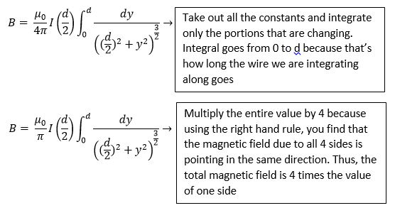
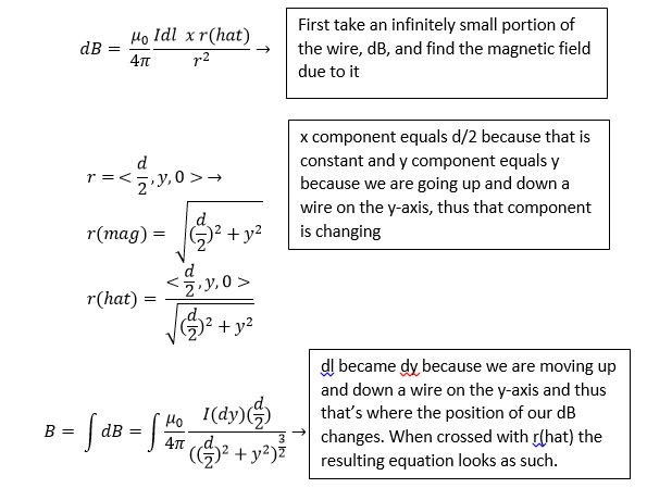
Simple
Middling
Hard
Connection
Calculus was invented to do physics. By integrating over an object to find its magnetic field, you are performing one of the basic operations on which physics is founded on, which is used to derive other formulas. Additionally, using this method should allow you to find the magnetic field of any object, no matter its shape or size. However, calculus as a whole can be applied to a variety of different areas. Integration specifically is essentially used to find the sum of something with infinite parts. For example, I am an industrial engineer, so if given a function of the output of a machine in regards to time, I could use integration to find the total output of the machine, which can help me later on in efficiency calculations.
History
Isaac Newton and Gottfried Leibniz are the two men to whom the discovery of calculus is usually attributed to. However, both men thought of calculus in different ways. Newton thought of calculus with the variables x and y changing over time and computed the tangent of curves using finite velocities of these two variables. However, Leibniz thought of calculus in terms of dx and dy being the difference in close, successive values in a sequence. Because Leibniz used more uniform notation when creating calculus, today's calculus symbols and terms are typically based of Leibniz's original work.


