Problem Solving

Linear algebra can be used to solve large ohmic circuits. This page explains how to define the circuit problem in terms of a linear system that can be solved with computational methods like matlab or python.

The Main Idea

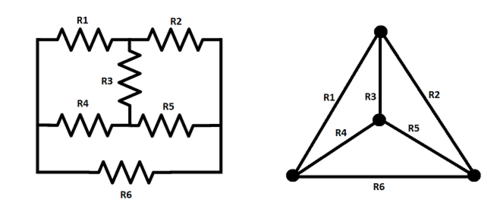
We can describe an electrical circuit as a graph where the nodes represent specific points and the edges represent the components connecting them. E.g:

Graph representation of a circuit

Incidence Matrix

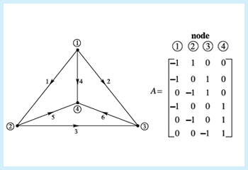
The incidence matrix, A, is a matrix of dimensions m x n, where m is the number of edges and n is the number of nodes. If x is the vector that contains all the nodes in order, A satisfies: [math]\displaystyle{ A\vec{x}_{edge} = x_{end} - x_{start} }[/math] Thus, the resulting matrix will have zeros in every element of each row, except for the start and the end nodes, which will be -1 and 1 respectively:

Incidence matrix of a sample graph.

Here, [math]\displaystyle{ x_{1}, x_{2}, x_{3} }[/math] and [math]\displaystyle{ x_{4} }[/math] represent the voltages at the nodes. Then [math]\displaystyle{ A\vec{x}_{edge} = x_{end} - x_{start} }[/math] gives the voltage differences [math]\displaystyle{ ∆V }[/math].

Loop Rule (Kirchhoff's voltage law)

Using this creative way of transforming a circuit to a graph and getting the incidence matrix from it allows us to do some interesting things. Kirchhoff's loop rule is a principle of conservation of energy that implies that the directed sum of the voltage differences around any closed network is zero.

This means that the components of [math]\displaystyle{ A\vec{x} = b }[/math] add to zero around every loop. Moreover, the voltage law can decide whether b is in the column space of A.

We know from Ohm's law that [math]\displaystyle{ V = I * R }[/math]. Then, in the previous graph for example, we would have that [math]\displaystyle{ V_{edge1} = I * R = (direction) * R_{1} = 1 * R_{1} }[/math].

Kirchhoff's Current Law

We know from Kirchhoff's law that the sum of the currents in each node is zero. This means that the current flowing into the node is the same as the current flowing out of the node. Therefore the multiplication of each column of A by the current vector, y, must be equal to zero:

[math]\displaystyle{ A^{T}\vec{y} = 0 }[/math]

where [math]\displaystyle{ y_{i} }[/math] is the current passing through edge [math]\displaystyle{ i }[/math].

If a circuit has a source like a battery, we can treat the entire circuit as a node. The current in and out of every node within the circuit will be zero except for the nodes connected to the positive and negative ends of the battery. For the positive end the net current, [math]\displaystyle{ S }[/math], will be positive and for the negative end the net current will be negative. Thus we get:

[math]\displaystyle{ A^{T}\vec{y} = f }[/math]

where [math]\displaystyle{ f_{i} = 0 }[/math] if [math]\displaystyle{ i }[/math] is not one of the nodes connected to the battery,[math]\displaystyle{ f_{i} = S }[/math] if [math]\displaystyle{ i }[/math] is connected to the positive end and [math]\displaystyle{ f_{i} = -S }[/math] if [math]\displaystyle{ i }[/math] is connected to the negative end.

Solving Problems

From Ohm's law we have [math]\displaystyle{ V = I * R }[/math]. Thus if we define the conductance diagonal matrix [math]\displaystyle{ C }[/math] where [math]\displaystyle{ C_{i,i} = \frac{1}{R_{i}} }[/math], [math]\displaystyle{ C_{i,j} = 0 }[/math], Ohm's law becomes:

[math]\displaystyle{ \vec{y} = -CA\vec{x} }[/math]

where [math]\displaystyle{ y_{i} }[/math] is the current through edge [math]\displaystyle{ i }[/math] and [math]\displaystyle{ x_{j} }[/math] is the voltage at node [math]\displaystyle{ j }[/math] . Substituting for y in Kirchhoff's law, we get:

[math]\displaystyle{ -A^{T}CA\vec{x} = f }[/math]

We can now use this system of matrices to solve circuit problems.

It is important to note that for the exercises posted above, the solutions for those problems should be easy to compute given the number of nodes and connections. Nevertheless, bigger and more complex problems would benefit massively from the methods of linear algebra, as they could be computed in this standard way.

Example

Suppose we have the following circuit (along with its graph and matrix representation):

Graph representation of a circuit

Solving the system, we get:

Notice that [math]\displaystyle{ C }[/math] is the identity, thus:

Solving for x, we get:

Connectedness

1. How is this topic connected to something that you are interested in?
2. How is it connected to your major?
3. Is there an interesting industrial application?

See also

Are there related topics or categories in this wiki resource for the curious reader to explore? How does this topic fit into that context?

Further reading

• Linear Algebra applications in image compression: https://math.mit.edu/~gs/linearalgebra/linearalgebra5_7-1.pdf

External links

Gilbert Strang's "Equilibrium Equations and Minimum Principles": http://cns-web.bu.edu/~eric/EC500/attachments/ON(2d)LINE(20)READINGS/strang.pdf

References

• Strang, G. (2016), Introduction to Linear Algebra, Wellesley-Cambridge Press, 5th edition, isbn:978-0-9802327-7-6