Iterative Prediction

This page describes iterative prediction, a technique used to predict the motion of particles over a period of time often used in simulations.

The Main Idea

Iterative prediction is a mathematical technique for approximating the behavior of one or more particles over an interval of time. To perform iterative prediction, the initial position, initial momentum, and mass of each particle must be known, and the forces acting on each particle must be known. Iterative prediction is not 100% accurate, but it is a very powerful tool because it can model complex systems that are impossible to model using known analytical approaches such as calculus.

To perform iterative prediction, the time interval of interest must be divided into small sub-intervals of duration [math]\displaystyle{ \Delta t }[/math] called time steps. For each time step, the following steps should be performed:

1. The net force acting on each particle should be calculated,
2. The linear momentum of each particle should be updated from the last time step using the newly calculated net force, and
3. The position of each particle should be updated from the last time step using its newly calculated velocity.

The size of the time steps used during iterative prediction is called the resolution of the model. Dividing a time interval into a few large time steps is called low resolution, while dividing the same time interval into many small time steps is called high resolution. Performing iterative prediction with a higher resolution produces more accurate results but requires more computations. This is because steps 2 and 3 assume constant force and velocity respectively during the duration of each time step. In reality, force and velocity change continually, so this is where inaccuracy is introduced. However, if the time steps are small enough that force and velocity do not significantly change during any time step, iterative prediction is a sufficiently accurate model. In the limit where the time interval is divided into an infinite number of infinitely small time steps, iterative prediction becomes a perfectly accurate model. However, this would require an infinite number of computations, and is therefore impossible to do, although in some simple situations, calculus can be used to this end instead. Deciding what time step to use requires consideration of both the computational resources available and the resolution required to accurately approximate the situation. When performing iterative prediction by hand, it is impractical to perform more than a few time steps, which cannot be used to accurately model much. If computers are available, it becomes feasible to divide the time interval into thousands of time steps, which can accurately simulate most day-to-day situations. Some of the most sensitive simulations, however, require incredibly small time steps. For example, some physicists perform atom-by-atom simulations of molecular structures interacting. A slight change in the position of an atom can cause a huge change in the forces acting on it, so tiny time steps must be used in order to ensure that force and velocity do not significantly change during any one time step. These simulations are run on the world's most powerful supercomputers and often take weeks to complete. They can simulate time intervals of several nanoseconds ([math]\displaystyle{ 10^{-9} }[/math] s) using time steps of only a few femtoseconds. ([math]\displaystyle{ 10^{-15} }[/math] s) (Click here for an example of a paper about such a simulation.)

A Mathematical Model

Below are the mathematical formulas required for each of the three steps above.

1. The net force acting on each particle should be calculated.
This step varies widely from program to program. Sometimes, the forces acting on each particle are constant, such as when modeling the motion of a ball with a specific weight thrown near the surface of the earth. Other times, the forces are functions of the particles' positions, such as when modeling the motion of celestial bodies whose gravitational attraction is greater when they are closer together. Sometimes, there is only one force acting on each particle, and other times, the net force must be found by adding together the individual force vectors.
2. The momentum of each particle should be updated from the last time step using the newly calculated net force.
This step uses the impulse-momentum theorem (see impulse and momentum). The impulse-momentum theorem states that [math]\displaystyle{ \vec{p}_f = \vec{p}_i + \vec{J} = \vec{p}_i + \vec{f}_{net, avg} * \Delta t }[/math]. In iterative prediction, the initial momentum is always known; it is simply the momentum the particle had during the previous time step (or, if there is no previous time step, the initial momentum of the particle). [math]\displaystyle{ \vec{f}_{net, avg} }[/math] represents the average net force that has been acting on the particle since the previous time step, resulting in a new momentum this time step. To calculate it, the net force found in step 1 should be used. Note that in reality, the net force acting on the particle is constantly changing, and the net force found in step 1 is the final net force, which is not truly the average net force over the course of the previous time step (except in a scenario with constant force). As described in the introductory section, this introduces inaccuracy that can be reduced by using shorter time steps; if short time steps are used, the net force does not have much time to change over the course of the time step, meaning the average net force is very similar to the final net force.
3. The position of each particle should be updated from the last time step using its newly calculated velocity.
This step uses the kinematic equation [math]\displaystyle{ \vec{r}_f = \vec{r}_i + \vec{v}_{avg} * \Delta t }[/math]. In iterative prediction, the initial position is always known; it is simply the position the particle had during the previous time step (or, if there is no previous time step, the initial position of the particle). [math]\displaystyle{ \vec{v}_{avg} }[/math] represents the average velocity with which the particle has been moving since the previous time step, resulting in a new position this time step. To calculate it, the momentum found in step 2 should simply be divided by the mass of the particle: [math]\displaystyle{ \vec{v}_f = \frac{\vec{p}_f}{m} }[/math]. Substituting this into the original formula yields [math]\displaystyle{ \vec{r}_f = \vec{r}_i + \frac{\vec{p}_f}{m} * \Delta t }[/math]. Note that in reality, the velocity of the particle is constantly changing, and the velocity found above is the final velocity, which is not truly the average velocity over the course of the previous time step (even in a scenario with constant force). As described in the introductory section, this introduces inaccuracy that can be reduced by using shorter time steps; if short time steps are used, the velocity does not have much time to change over the course of the time step, meaning the average velocity is very similar to the final velocity.

A Computational Model

Iterative prediction is typically done on computers because many computations are necessary in order to perform it with a meaningful resolution. Below is an example of a vPython program that uses iterative prediction to simulate a ball thrown near the surface of the earth:

high resolution simulation

To demonstrate differing resolutions, here is a lower resolution version of the same simulation, which uses larger time steps:

low resolution simulation

Note that the first program is more realistic; the more frequent position updates result in a smoother curve that more closely approximate the true trajectory of a ball. On the other hand, the second program has fewer calculations to do. Both programs are artificially slowed using the "rate" command in order to simulate a realistic travel time, but if both programs were allowed to run as quickly as possible, the second program would finish first. For larger, more complicated simulations, time can be a significant factor.

Example Calculations

There are a variety of different problems that can be solved by utilizing the momentum update form of the Momentum Principle. They can vary in difficulty and require any number of iterations. It is often prudent to calculate these iterations in a program loop to save time and avoid miscalculations.

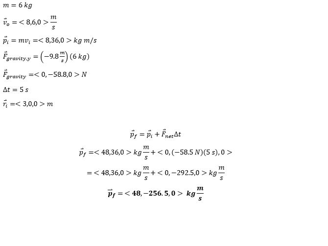
Example #1 - Momentum Update

A 6kg ball is thrown into the air with an initial velocity of [math]\displaystyle{ {\lt 8,6,0\gt m/s} }[/math]. If the only force acting on the ball is gravity, what is the final momentum of the ball after 5 seconds?

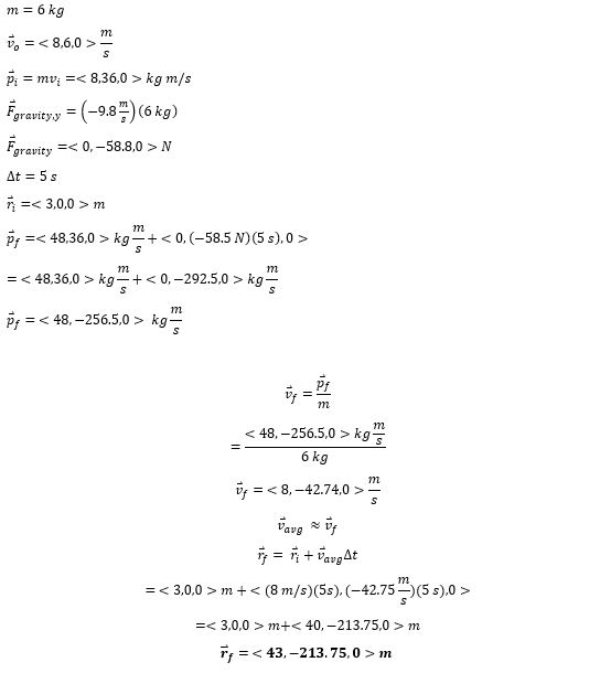
Example #2 - Trajectory Maxima

A 6kg ball is thrown into the air with an initial velocity of [math]\displaystyle{ {\lt 8,6,0\gt m/s} }[/math] and the only force acting on the ball is gravity. What is it's position after 5 seconds if it started out at [math]\displaystyle{ {\lt 3, 0 ,0\gt m} }[/math]?

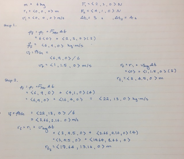
Example #3 - Varying Force

A 6kg ball is sitting at [math]\displaystyle{ {\lt 0, 0,0\gt m} }[/math]. If the ball was kicked with a force of[math]\displaystyle{ {\lt 2,3,0\gt N} }[/math], and then kicked with a force of [math]\displaystyle{ {\lt 4,1,0\gt N} }[/math] 3 seconds later, how far did it travel after an additional 4 seconds?

Connectedness

Iterative prediction is interesting to me in that modeling its motion on a computer can be both complex and very simple. The idea that with a powerful processor you can get infinitely more accurate results than on a laptop is amazing. How much more accurate would our VPython be in lab? Does this mean that our VPython models are erroneous by miniscule amount? Beyond the process of answers, the idea that we are essentially "predicting the future" through math is exciting and really opens up a lot of questions as to the limit of what is predictable and what is not. The most simple idea resulting from iterative prediction is the principle of "this is where I started from, what will it take to get to here" or "this is where I started, where will I end up if I". As a biochemistry major, this principle is a large part of my laboratory procedures. Each reaction that I have to create isn't a blind "let's put in this much of reactant A with B and see how much C I end up with". It's always a question of calculating how much reactant is needed to complete the first reaction, as well calculating the results of what the product will be if this much reactant is added. For complex multi-step reactions, it's identical to the momentum update principle in that you are constantly taking what you are given and solving for where you end up after each reaction to get to the expected final product. Iterative prediction would be useful in pharmaceutical companies that are always trying to determine the effects of medications at the first instance of ingestion, and as the medicine dissolves (several reactions) in the stomach. Essentially, they would be creating multi-step reactions to simulate the human stomach in order to determine if the medication was performing as it should/not being detrimental towards our bodies.

History

The physics behind iterative prediction is nothing more than simple application of the momentum principle and projectile motion, which has existed in classical mechanics for quite some time. However, the practical application of iterative prediction for analyzing systems has evolved due to advances in computational methods and technology. With the computational power of a computer to iteratively calculate changes in momentum through time, one can analyze a system's motion extremely quickly without tedious and difficult mathematical calculations.

See also

There are many public resources that delve further into iterative prediction examples of more complex motion.

External links

Physics Portal

HyperPhysics Concept Map

MIT Open Courseware Introductory Mechanics

Iterative Prediction with VPython

References

CHANGE LECTURE SLIDES Georgia Institute of Technology. Physics Department. PHYS 2211. Fall 2016. Wednesday, Week 2 Lecture Slides. Fenton, Flavio H

Georgia Institute of Technology. Physics Department. PHYS 2211. Fall 2016. Monday, Week 3 Lecture Slides. Fenton, Flavio H

Georgia Institute of Technology. Physics Department. PHYS 2211. Fall 2016. Lab 07 Fancart Energy & Spring-Mass Instructions, Greco, Edwin

http://p3server.pa.msu.edu/coursewiki/doku.php?id=183_notes:iterativepredict

https://www.ncbi.nlm.nih.gov/pmc/articles/PMC6286305/ (fix up this citation)