Electric Field

The Main Idea

CYNTHIA MILLER (FALL 2020)

Here, the concept of an Electric Field produced by a point charge is explored qualitatively and quantitatively through models, examples, and a simulation. An Electric Field is a useful concept to describe how any charged particle or collection of charged particles (positive / negative would affect surrounding charge.

The Electric Field of a point charge is spherically symmetric, (same at all points of equal radius from the source. Hence, it is useful to speak of the electric field at a certain radius (not at a certain [math]\displaystyle{ (x,y,z) }[/math] position), which is explained in the mathematical model.

Keep in mind, the electric field is a vector quantity, meaning it has a magnitude and direction. The SI units are N/C.

A Mathematical Model

The Electric Field vector [math]\displaystyle{ \bigl( \mathbf{E}_{s} \bigl) }[/math] of a point source charge [math]\displaystyle{ \bigl( Q_{s} \bigl) }[/math] gives the magnitude and direction of the Electrostatic Force vector [math]\displaystyle{ \bigl( \mathbf{F}_{s} \bigl) }[/math] exerted on a unit charge ([math]\displaystyle{ 1 }[/math] Coulomb) by [math]\displaystyle{ Q_{s} }[/math], as a function of position [math]\displaystyle{ \bigl( \mathbf{r} = (x,y,z) \bigl) }[/math]. More generally however, the Electrostatic Force vector exerted on any point charge [math]\displaystyle{ \bigl( q \bigl) }[/math] by a point source charge [math]\displaystyle{ \bigl( Q_{s} \bigl) }[/math] is related to the source charge's Electric Field vector by:

[math]\displaystyle{ \mathbf{F}_{s} ( \mathbf{r} ) = q \mathbf{E}_{s} ( \mathbf{r} ) }[/math]

This definition requires an understanding of the Electrostatic Force (Coulomb's Law), and its mathematical description. If you are not familiar with this yet, read over the Electric Force page and come back.

Since the Electric Force is defined as:

[math]\displaystyle{ \mathbf{F}( \mathbf{r} ) = \frac{1}{4\pi\epsilon_{o}}\frac{q_{1} q_{2}}{r^{2}} \hat{\mathbf{r}} }[/math], where

[math]\displaystyle{ \epsilon_{o} }[/math] is the permittivity of free space with a value of [math]\displaystyle{ 8.854 \times 10^{-12} \frac{\text{C}^2}{\text{N} \cdot \text{m}^2} }[/math]

[math]\displaystyle{ q_{1} }[/math] and [math]\displaystyle{ q_{2} }[/math] are two different point charges

[math]\displaystyle{ r }[/math] is the distance between the two point charges, which can also be written as [math]\displaystyle{ |\mathbf{r}| }[/math], the magnitude of the vector connecting the two charges' positions

[math]\displaystyle{ \hat{\mathbf{r}} }[/math] is the unit vector pointing from charge one to charge two, or from charge two to charge one, depending on whether the force on charge two or charge one is sought for.

The Electric Field of a source charge [math]\displaystyle{ Q_{s} }[/math] is:

[math]\displaystyle{ \begin{align} \mathbf{E}_{s} ( \mathbf{r}) & = \frac{\mathbf{F}_{s} ( \mathbf{r} )}{q} \\ & = \frac{1}{4\pi\epsilon_{o}}\frac{Q_{s}}{r^{2}}\hat{\mathbf{r}} \end{align} }[/math]

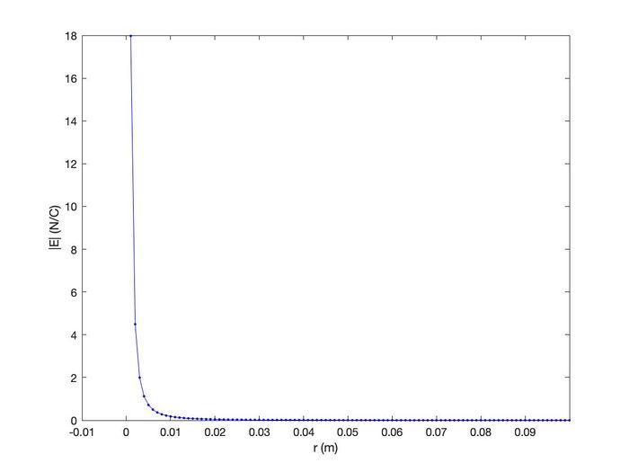
As evidently based from the mathematical formula of an electric field for a point charge (which can also be applied to a spherically uniformly charged body), the electric field has an inverse-square relationship with the radius regarding the observation location. Essentially, as distance (radius) increases from the point charge's source, it's electric field at that observation location weakens by a corresponding factor of [math]\displaystyle{ {r^{-2}} }[/math]

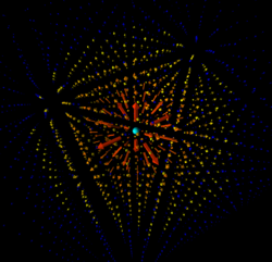
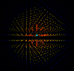
Radially, the magnitude of a point charge's Electric Field looks something like this:

[math]\displaystyle{ 2 \times 10^{-15} \ \text{C} }[/math] charge's Electric Field magnitude as a function of radius.

A point charge's Electric Field is also related to its Electric Potential. If you are unfamiliar with the idea of electric potential, then review these pages (Electric Field and Electric Potential and Electric Potential) and come back.

A charge's Electric Field and Electric Potential [math]\displaystyle{ V }[/math] are related by:

[math]\displaystyle{ V_{ab} = -\int_{\mathbf{b}}^{\mathbf{a}} \mathbf{E} \cdot d\mathbf{L} }[/math], where

[math]\displaystyle{ V_{ab} }[/math] is the potential difference between points [math]\displaystyle{ \mathbf{a} }[/math] and [math]\displaystyle{ \mathbf{b} }[/math]

[math]\displaystyle{ \mathbf{E} }[/math] is the Electric Field

[math]\displaystyle{ d\mathbf{L} }[/math] is an infinitesimal length along the path between [math]\displaystyle{ \mathbf{a} }[/math] and [math]\displaystyle{ \mathbf{b} }[/math]

This relation is less useful for us unless we use a straight line approximation, such that:

[math]\displaystyle{ \begin{align} V_{ab} & = -\mathbf{E} \cdot \Delta \mathbf{L} \\ & = - \bigl( E_{x}, E_{y}, E_{z} \bigl) \cdot \bigl( \Delta L_{x}, \Delta L_{y}, \Delta L_{z} \bigl) \\ & = - \bigl( E_{x}\Delta L_{x} + E_{y}\Delta L_{y} + E_{z}\Delta L_{z} \bigl) \\ \end{align} }[/math]

This leads to:

[math]\displaystyle{ \mathbf{E} (x,y,z) = - \biggl( \frac{\Delta V_{x}}{\Delta L_{x}}, \frac{\Delta V_{y}}{\Delta L_{y}}, \frac{\Delta V_{z}}{\Delta L_{z}} \biggl) }[/math]

By convention, the Electric Field due to a positive point charge always points away from itself, and the Electric Field of a negative point charge always points towards itself as shown below:

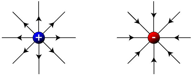
Opposite charges will attract each other, and like charges will repel each other, as shown below:

Lastly, the Principle of Superposition is directly applicable to finding the Electric Field due to multiple point source charges, using the a vector sum:

[math]\displaystyle{ \begin{align} \mathbf{E}_{sum} (\mathbf{r}) & = \mathbf{E}_{1} + \mathbf{E}_{2} + \mathbf{E}_{3} + \cdots + \mathbf{E}_{N} \\ & = \sum_{1}^{N} \mathbf{E}_{n} \\ & = \sum_{1}^{N} \frac{1}{4 \pi \epsilon_{o}} \frac{Q_{s_{n}}}{r_{n}^{2}} \hat{\mathbf{r}}_n \end{align} }[/math]

• When using this, be careful to take note that the Electric Field of a negative charge points in the opposite direction as a positive charge.

• Critical Formulas:
  • [math]\displaystyle{ \mathbf{E} ( \mathbf{r}) = \frac{\mathbf{F} ( \mathbf{r} )}{q} }[/math]
  • [math]\displaystyle{ \mathbf{E} ( \mathbf{r}) = \frac{1}{4\pi\epsilon_{o}}\frac{Q}{r^{2}}\hat{\mathbf{r}} }[/math]
  • [math]\displaystyle{ \mathbf{E} (x,y,z) = - \biggl( \frac{\Delta V_{x}}{\Delta L_{x}}, \frac{\Delta V_{y}}{\Delta L_{y}}, \frac{\Delta V_{z}}{\Delta L_{z}} \biggl) }[/math]
  • [math]\displaystyle{ \mathbf{E}_{sum} (\mathbf{r}) = \sum_{1}^{N} \frac{1}{4 \pi \epsilon_{o}} \frac{Q_{s_{n}}}{r_{n}^{2}} \hat{\mathbf{r}}_n }[/math]

Normal view of simulated electric field

A Computational Model

   ###--Create Electric Field Lines of a Positive Charge at the Origin--###
   #==============================================================#
   #---Import statements for VPython---#
   from __future__ import division
   from visual import *
   #---Import function used to find combinations---#
   from itertools import combinations
   #==============================================================#
   #---Create scene---#
   scene.center = vector(0,0,0)  #-Position of source charge-#
   scene.height = 800  #-Set height of frame of scene-#
   scene.width = 800  #-Set width of frame of scene-#
   scene.range = 4  #-Set range of scene-#
   scene.userzoom = 1  #-Allow user to zoom in/out: CTRL & move in/out on trackpad-#
   scene.userspin = 1  #-Allow user to rotate camera angle: SHIFT & OPTION & move around on track pad-#
   #==============================================================#
   #---Specify point charge attributes---#
   sourceCharge = 3*10**(-11)  #-Coulombs of charge-#
   sourcePos = vector(0,0,0) #-Position of source charge-#
   ###--Modeling source point charge as a sphere with radius 0.1 meters--###
   sourceObj = sphere(pos = sourcePos, radius = 0.1, color = color.cyan)
   #==============================================================#
   #---Set range (0 to 3) and possible inputs for the coordinates (0.5 step)---#
   ###--Many of the same number included to allow for combinations such as (1,1,1).
       #The itertools.combinations function will only use each element of the...
       #list once, starting from the beginning.
       #Repeating each coordinate many times with intermixing, grants...

Distant view of simulated electric field

       #all combinations of points, with repeats however.
       #Later, a for loop will be used to eliminate repeats.
       #This can be optimized later if need be.---------------###
   posXYZ = [0, -0.5, 1, -1.5, 2, -2.5, 3,
             0, 0.5, -1, 1.5, -2, 2.5, -3,
             0, -0.5, 1, -1.5, 2, -2.5, 3,
             0, 0.5, -1, 1.5, -2, 2.5, -3,
             0, -0.5, 1, -1.5, 2, -2.5, 3,
             0, 0.5, -1, 1.5, -2, 2.5, -3,
             0, -0.5, 1, -1.5, 2, -2.5, 3,
             0, 0.5, -1, 1.5, -2, 2.5, -3,
             0, -0.5, 1, -1.5, 2, -2.5, 3,
             0, 0.5, -1, 1.5, -2, 2.5, -3,
             0, -0.5, 1, -1.5, 2, -2.5, 3,
             0, 0.5, -1, 1.5, -2, 2.5, -3]
   #==============================================================#

Rotated and zoomed in view of simulated electric field

   #---Create combinations of points (x,y,z) for later use---#
       ###--prelimPoints will be a list of tuples of tuples--##
           #ie: [((,,),(,,),(,,),(,,)) , ((,,),(,,)) ,..., ((,,),(,,))]
   prelimPoints = [tuple(combinations(posXYZ, 3))]
   ###--Pull the points out of the grouping tuples and add them to a...
       #new list alphaPoints------------------------###
   alphaPoints = []
   for groupingTuple in prelimPoints:
       for XYZ in groupingTuple:
           if XYZ not in alphaPoints:  #-Check for repeat (x,y,z)-#
               alphaPoints.append(XYZ)
           ##--The negative of this tuple may not be in the combinations:
               #check to see-------------##
           first = -XYZ[0]
           second = -XYZ[1]
           third = -XYZ[2]
           negXYZ = (first, second, third)
           if negXYZ not in alphaPoints:
               alphaPoints.append(negXYZ)
           ##--Swap x and z coordinates for futher combination checking--##
           first = XYZ[2]
           second = XYZ[1]
           third = XYZ[0]
           reverseXYZ = (first, second, third)
           if reverseXYZ not in alphaPoints:
               alphaPoints.append(reverseXYZ)
           ##--The negative of the x and z coordinate swap may not be in...
               #the combinations: check to see---------##
           first = -XYZ[2]
           second = -XYZ[1]
           third = -XYZ[0]
           reverseXYZneg = (first, second, third)
           if reverseXYZneg not in alphaPoints:
               alphaPoints.append(reverseXYZneg)
           ##--Make x [3], y [0], and z [1] to check for more combinations--##
           first = XYZ[1]
           second = XYZ[2]
           third = XYZ[0]
           shiftedXYZ = (first, second, third)
           if shiftedXYZ not in alphaPoints:
               alphaPoints.append(shiftedXYZ)
           ##--The negative of the shifted XYZ may not be in the combinations:
               #check to see---------------##
           first = -XYZ[1]
           second = -XYZ[2]
           third = -XYZ[0]
           shiftedXYZneg = (first, second, third)
           if shiftedXYZneg not in alphaPoints:
               alphaPoints.append(shiftedXYZneg)
   ###--------This should be enough recombining---------###
   #================================================================#

Rotated top view of simulated electric field

   #---Create a new list of tuples that contain the points, magnitude,...
       #and direction (betaPoints)-----------#
           #ie: [((x,y,z), mag((x,y,z)), norm((x,y,z))),...]
   betaPoints = []
   for XYZ in alphaPoints:
       Mag = mag(XYZ)
       Dir = norm(XYZ)
       betaPoints.append((XYZ, Mag, Dir))
   #================================================================#
   #---Sort the tuples based on their magnitudes from least to greatest...
      #using sorted().
           #key = lamda x: x[1] tells the sorted function to sort the tuples...
               #based on their second component...their magnitudes--------#
   charliePoints = sorted(betaPoints, key = lambda x: x[1])
   #================================================================#
   #---Calculate parts of electric field equation:
       #E = 1/(4*pi*epsilon0) * Q/(magnitude)**2
   epsilonO = 8.854*(10**(-12)) #-N*(m/C)**2-#
   k = 1/(4*pi*(epsilonO)) #-N*(m/C)**2-#
   chargeContri = k*sourceCharge #-N*(m**2/C)-#
   #================================================================#
   #---Loop through points and find mag of electric field:
       #add it to a new list with the existing tuple info-------#
   deltaPoints = []
   for XYZ in charliePoints:
       try:  ###-Avoid divide by 0 error in (x,y,z) = (0,0,0)-###
           magEfield = chargeContri*(1/(XYZ[1])**2)
       except:
           magEfield = 0
       tupEfield = (XYZ[0], XYZ[1], XYZ[2], magEfield)
       deltaPoints.append(tupEfield)
   #================================================================#

Side angle of simulated electric field

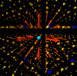
   #---Loop through points and create an arrow at that point proportional in...
       #length to the magnitude of the electric field there.
       #Also, the arrow points in the direction of the electric field there.
       #Color coding is based on 0.25 meter increments:
           #stronger field = redder; weaker field = blue
   for XYZ in deltaPoints:
       if XYZ[1] <= 0.25:
           lengthP = XYZ[3]*0.5
           arroW = arrow(pos=vector(XYZ[0]), axis=XYZ[2],
                         color = vector(1.000, 0.000, 0.000),
                         length = lengthP,
                         headwidth = lengthP*0.2,
                         headlength = lengthP*0.25)
       elif XYZ[1] <= 0.5:
           lengthP = XYZ[3]*0.7
           arroW = arrow(pos=vector(XYZ[0]), axis=XYZ[2],
                         color = vector(1.000, 0.200, 0.000),
                         length = lengthP,
                         headwidth = lengthP*0.2,
                         headlength = lengthP*0.25)
       elif XYZ[1] <= 1:
           lengthP = XYZ[3]*0.9
           arroW = arrow(pos=vector(XYZ[0]), axis=XYZ[2],
                         color = vector(1.000, 0.300, 0.000),
                         length = lengthP,
                         headwidth = lengthP*0.2,
                         headlength = lengthP*0.25)
       elif XYZ[1] <= 1.25:
           lengthP = XYZ[3]*1.1
           arroW = arrow(pos=vector(XYZ[0]), axis=XYZ[2],
                         color = vector(1.000, 0.400, 0.000),
                         length = lengthP,
                         headwidth = lengthP*0.2,
                         headlength = lengthP*0.25)
       elif XYZ[1] <= 1.5:
           lengthP = XYZ[3]*1.3
           arroW = arrow(pos=vector(XYZ[0]), axis=XYZ[2],
                         color = vector(1.000, 0.500, 0.000),
                         length = lengthP,
                         headwidth = lengthP*1,
                         headlength = lengthP*1)
       elif XYZ[1] <= 1.75:
           lengthP = XYZ[3]*1.5
           arroW = arrow(pos=vector(XYZ[0]), axis=XYZ[2],
                         color = vector(1.000, 0.600, 0.000),
                         length = lengthP,
                         headwidth = lengthP*1,
                         headlength = lengthP*1)
       elif XYZ[1] <= 2:
           lengthP = XYZ[3]*1.7
           arroW = arrow(pos=vector(XYZ[0]), axis=XYZ[2],
                         color = vector(1.000, 0.700, 0.000),
                         length = lengthP,
                         headwidth = lengthP*1,
                         headlength = lengthP*1)
       elif XYZ[1] <= 2.25:
           lengthP = XYZ[3]*1.9
           arroW = arrow(pos=vector(XYZ[0]), axis=XYZ[2],
                         color = vector(1.000, 0.800, 0.000),
                         length = lengthP,
                         headwidth = lengthP*1,
                         headlength = lengthP*1)
       elif XYZ[1] <= 2.5:
           lengthP = XYZ[3]*2.1
           arroW = arrow(pos=vector(XYZ[0]), axis=XYZ[2],
                         color = vector(1.000, 0.900, 0.000),
                         length = lengthP,
                         headwidth = lengthP*1,
                         headlength = lengthP*1)
       elif XYZ[1] <= 2.75:
           lengthP = XYZ[3]*2.3
           arroW = arrow(pos=vector(XYZ[0]), axis=XYZ[2],
                         color = vector(1.000, 1.000, 0.000),
                         length = lengthP,
                         headwidth = lengthP*1,
                         headlength = lengthP*1)
       else:
           lengthP = XYZ[3]*2.5
           arroW = arrow(pos=vector(XYZ[0]), axis=XYZ[2],
                         color = color.blue,
                         length = lengthP,
                         headwidth = lengthP*1,
                         headlength = lengthP*1)

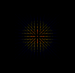
• This link Charges and Fields provides a PhET simulation of Electric Fields. Play with it!

• Or if you prefer something with more action, explore this Hockey Game to gain a deeper visual understanding of electric fields and their effects on charges

Examples

Simple

• Question:

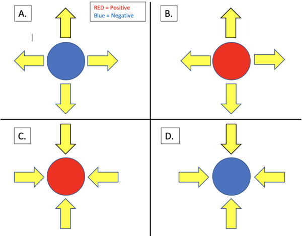
In the following figure, the red circles represent positive point charges, and the blue circles represent negative point charges. If the yellow arrows are meant to represent the Electric Field due to each point charge, which field(s) and charge(s) are correctly matched? (Only take into account direction)

• Solution:

Since Electric Field lines always point away from a positive point charge, Option (C.) cannot be correct. Likewise, Electric Field lines always point towards a negative charge. Therefore, Option (A.) is also incorrect.

Option (B.) shows a positive charge with an Electric Field pointing radially outwards. This is correct. Option (D.) shows a negative charge with an Electric Field pointing radially inwards. This is also correct.

Answer: Options (B.) & (D.)

Middling

• Question:

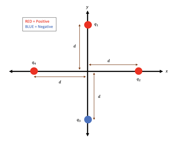
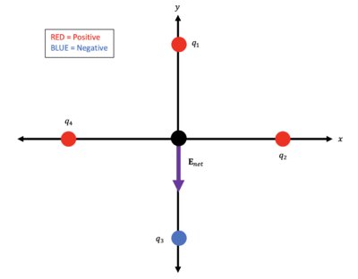
Four point charges [math]\displaystyle{ \big(q_{1}, q_{2}, q_{3}, \text{and} \ q_{4} \big) }[/math], are each located at a distance [math]\displaystyle{ d }[/math] along either the [math]\displaystyle{ x }[/math] or [math]\displaystyle{ y }[/math] axes, as shown in the figure below.

• A.) What is the net Electric Field at the origin?
• B.) If [math]\displaystyle{ \ |q_{3}| = |q_{1}| \ \text{and} \ |q_{4}| = |q_{2}| }[/math] what does the Electric Field at the origin reduce to?

• Solution:

• A.) To find the net Electric Field at the origin, we must first find the Electric Field due to each charge at the origin.

• Starting with [math]\displaystyle{ q_{1} }[/math], its general Electric Field can be described as:

[math]\displaystyle{ \mathbf{E}_{1} = \frac{1}{4 \pi \epsilon_{0}} \frac{|q_{1}|}{r_{1}^2} \hat{\mathbf{r}}_{1} }[/math]

[math]\displaystyle{ r_{1} }[/math] is measured relative to the location of [math]\displaystyle{ q_{1} }[/math].

The origin is a distance [math]\displaystyle{ d }[/math] away from [math]\displaystyle{ q_{1} }[/math], which is along the y-axis. Since it is a positive charge, its Electric Field at the origin will point "down" the y-axis (away from the charge):

[math]\displaystyle{ \mathbf{E}_{1} = \frac{1}{4 \pi \epsilon_{0}} \frac{|q_{1}|}{d^2} (-\mathbf{j}) }[/math] where [math]\displaystyle{ \mathbf{j} }[/math] is the unit vector in the y-direction.

• For [math]\displaystyle{ q_{2} }[/math] we have:

[math]\displaystyle{ \mathbf{E}_{2} = \frac{1}{4 \pi \epsilon_{0}} \frac{|q_{2}|}{r_{2}^2} \hat{\mathbf{r}}_{2} }[/math]

[math]\displaystyle{ r_{2} }[/math] is measured relative to the location of [math]\displaystyle{ q_{2} }[/math].

The origin is a distance [math]\displaystyle{ d }[/math] away from [math]\displaystyle{ q_{2} }[/math], which is along the x-axis. Since it is a positive charge, its Electric Field at the origin will point to the left (away from the charge):

[math]\displaystyle{ \mathbf{E}_{2} = \frac{1}{4 \pi \epsilon_{0}} \frac{|q_{2}|}{d^2} (-\mathbf{i}) }[/math] where [math]\displaystyle{ \mathbf{i} }[/math] is the unit vector in the x-direction.

• For [math]\displaystyle{ q_{3} }[/math] we have:

[math]\displaystyle{ \mathbf{E}_{3} = \frac{1}{4 \pi \epsilon_{0}} \frac{|q_{3}|}{r_{3}^2} \hat{\mathbf{r}}_{3} }[/math]

[math]\displaystyle{ r_{3} }[/math] is measured relative to the location of [math]\displaystyle{ q_{3} }[/math].

The origin is a distance [math]\displaystyle{ d }[/math] away from [math]\displaystyle{ q_{3} }[/math], which is along the y-axis. Since it is a negative charge, its Electric Field at the origin will point "down" the y-axis (towards the charge):

[math]\displaystyle{ \mathbf{E}_{3} = \frac{1}{4 \pi \epsilon_{0}} \frac{|q_{3}|}{d^2} (-\mathbf{j}) }[/math] where [math]\displaystyle{ \mathbf{j} }[/math] is the same unit vector in the y-direction from earlier.

• For [math]\displaystyle{ q_{4} }[/math] the electric field is:

[math]\displaystyle{ \mathbf{E}_{4} = \frac{1}{4 \pi \epsilon_{0}} \frac{|q_{4}|}{r_{4}^2} \hat{\mathbf{r}}_{4} }[/math]

[math]\displaystyle{ r_{4} }[/math] is measured relative to the location of [math]\displaystyle{ q_{4} }[/math].

The origin is a distance [math]\displaystyle{ d }[/math] away from [math]\displaystyle{ q_{4} }[/math], which is along the x-axis. Since it is a positive charge, its Electric Field at the origin will point to the right (away from the charge):

[math]\displaystyle{ \mathbf{E}_{4} = \frac{1}{4 \pi \epsilon_{0}} \frac{|q_{4}|}{d^2} (\mathbf{i}) }[/math] where [math]\displaystyle{ \mathbf{i} }[/math] is the same unit vector in the x-direction from earlier.

Now that we have the four Electric Fields present at the origin, we can use the Principle of Superposition to find the net Electric Field at the origin:

[math]\displaystyle{ \begin{align} \mathbf{E}_{net} &= \mathbf{E}_{1} + \mathbf{E}_{2} + \mathbf{E}_{3} + \mathbf{E}_{4} \\ &= \frac{1}{4 \pi \epsilon_{0}} \frac{|q_{1}|}{d^2} (-\mathbf{j}) + \frac{1}{4 \pi \epsilon_{0}} \frac{|q_{2}|}{d^2} (-\mathbf{i}) + \frac{1}{4 \pi \epsilon_{0}} \frac{|q_{3}|}{d^2} (-\mathbf{j}) + \frac{1}{4 \pi \epsilon_{0}} \frac{|q_{4}|}{d^2} (\mathbf{i}) \\ &= \frac{1}{4 \pi \epsilon_{0} d^{2}} \Big[ -|q_{1}| \mathbf{j} -|q_{2}| \mathbf{i} -|q_{3}| \mathbf{j} + |q_{4}| \mathbf{i} \Big] \\ \mathbf{E}_{net} &= \frac{1}{4 \pi \epsilon_{0} d^{2}} \Big[ \big( |q_{4}| - |q_{2}| \big)\mathbf{i} - \big( |q_{1}| + |q_{3}| \big)\mathbf{j} \Big] \end{align} }[/math]

Part (B) answer

• B.) We will simply plug in the specified values into our answer from (A):

[math]\displaystyle{ \begin{align} \mathbf{E}_{net} &= \frac{1}{4 \pi \epsilon_{0} d^{2}} \Big[ \big( |q_{4}| - |q_{2}| \big)\mathbf{i} - \big( |q_{1}| + |q_{3}| \big)\mathbf{j} \Big] \\ &= \frac{1}{4 \pi \epsilon_{0} d^{2}} \Big[ \big( |q_{2}| - |q_{2}| \big)\mathbf{i} - \big( |q_{1}| + |q_{1}| \big)\mathbf{j} \Big] \\ &= \frac{1}{4 \pi \epsilon_{0} d^{2}} \Big[ 0 \mathbf{i} - 2|q_{1}| \mathbf{j} \Big] \\ &= \frac{1}{4 \pi \epsilon_{0} d^{2}} \Big[ - 2|q_{1}| \mathbf{j} \Big] \\ \mathbf{E}_{net} &= - \frac{1}{2 \pi \epsilon_{0} d^{2}} |q_{1}| \mathbf{j} \\ \end{align} }[/math]

Answer:

• A.) [math]\displaystyle{ \mathbf{E}_{net} = \frac{1}{4 \pi \epsilon_{0} d^{2}} \Big[ \big( |q_{4}| - |q_{2}| \big)\mathbf{i} - \big( |q_{1}| + |q_{3}| \big)\mathbf{j} \Big] }[/math]
• B.) [math]\displaystyle{ \mathbf{E}_{net} = - \frac{1}{2 \pi \epsilon_{0} d^{2}} |q_{1}| \mathbf{j} }[/math]

Difficult

• Question:

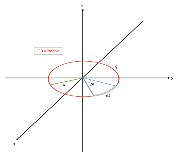
A ring of evenly distributed charge of radius [math]\displaystyle{ a }[/math] is centered on the origin in the xy-plane. The ring has a total charge [math]\displaystyle{ Q }[/math]. Show that the Electric Field due to this ring is 0 at the origin.

• Solution:

The Electric Field due to a point charge is given by:

[math]\displaystyle{ \mathbf{E} = \frac{1}{4 \pi \epsilon_{0}} \frac{|Q|}{| \mathbf{r} - \mathbf{r}^{'} |^{2}} \frac{\mathbf{r} - \mathbf{r}^{'}}{| \mathbf{r} - \mathbf{r}^{'} |} }[/math]

This equation is equivalent to the formula presented in the Mathematical Model. The reason it looks so different is due to a few assumptions in the mathematical model that we have stopped using:

1. The source charge is located at the origin (our ring of charge is around the origin)
2. The distance between the source charge and the observing location is simply expressed as a distance [math]\displaystyle{ r }[/math] (like in the Middling Example). Now, instead we will represent the distance as the magnitude of the difference in position between the source and observer [math]\displaystyle{ \big( | \mathbf{r} - \mathbf{r}^{'} | \big) }[/math].
3. Subsequently, our unit vector in the direction of the field [math]\displaystyle{ \big( \hat{\mathbf{r}} \big) }[/math] is not simply expressed as a typical unit vector (like in the middling example). It has now become the vector joining the source and observer divided by the magnitude of this same vector [math]\displaystyle{ \bigg( \frac{\mathbf{r} - \mathbf{r}^{'}}{| \mathbf{r} - \mathbf{r}^{'} |} \bigg) }[/math].

Another complication this problem presents is:

Where is the source charge?

To answer this, notice that the ring has an evenly distributed TOTAL charge [math]\displaystyle{ Q }[/math] and a radius [math]\displaystyle{ a }[/math]. Also, notice that the "source" position is constantly changing as you go around the ring. This issue makes it much more convenient to speak of the line charge DENSITY at a point along the ring instead of the TOTAL charge. This will allow us to treat the ring as many, many little source charges. The line charge density is simply the charge on the line divided by the length of that line (circumference), since the charge is evenly distributed about the ring:

[math]\displaystyle{ \rho_{L} = \frac{Q}{2 \pi a} }[/math]

This allows us to represent a differential amount of source charge as a product of the line charge density and a differential length:

[math]\displaystyle{ dQ = \rho_{L} dL }[/math]

The next question is: What is a differential length around the ring?

The differential length is a differential arc length [math]\displaystyle{ (s = r \theta) }[/math] around the circle dependent on the change in angle:

[math]\displaystyle{ dL = a d\theta }[/math]

Therefore:

[math]\displaystyle{ \begin{align} dQ &= \frac{Q}{2 \pi a} a d\theta \\ &= \frac{Q}{2 \pi} d\theta \\ \end{align} }[/math]

Now we can sum each of these differential source charge's contribution to the Electric Field at the origin using an integral:

[math]\displaystyle{ \mathbf{E} = \int \frac{1}{4 \pi \epsilon_{0}} \frac{\frac{Q}{2 \pi} d\theta}{| \mathbf{r} - \mathbf{r}^{'} |^{2}} \frac{\mathbf{r} - \mathbf{r}^{'}}{| \mathbf{r} - \mathbf{r}^{'} |} }[/math]

The only things left to find are the generic source position (a vector that can describe the position of each differential source charge along the ring) and the observer location. The observer location is given to us; the origin:

[math]\displaystyle{ \mathbf{r} = 0\mathbf{i} +0\mathbf{j} + 0\mathbf{k} }[/math]

The source position is easiest to describe as a radius from the origin (polar coordinates):

[math]\displaystyle{ \mathbf{r}^{'} = a \hat{ \mathbf{a}}_{r} }[/math] where [math]\displaystyle{ \hat{\mathbf{a}}_{r} }[/math] is a unit vector in the radial direction

Therefore:

[math]\displaystyle{ \begin{align} \mathbf{r} - \mathbf{r}^{'} &= \big( 0\mathbf{i} +0\mathbf{j} + 0\mathbf{k} \big) - \big( a\hat{ \mathbf{a}}_{r} \big) \\ &= -a\hat{ \mathbf{a}}_{r} \\ |\mathbf{r} - \mathbf{r}^{'}| &= \sqrt{(-a)^{2}} \\ &= a \\ \end{align} }[/math]

Plugging these into the Electric Field integral gives:

[math]\displaystyle{ \begin{align} \mathbf{E} &= \int \frac{1}{4 \pi \epsilon_{0}} \frac{\frac{Q}{2 \pi} d\theta}{a^2} \frac{-a \hat{ \mathbf{a}}_{r}}{a} \\ &= - \int \frac{1}{8 {\pi}^{2} \epsilon_{0}} \frac{Q}{a^2} \hat{ \mathbf{a}}_{r} d\theta \\ &= - \frac{Q}{a^{2} 8 {\pi}^{2} \epsilon_{0}} \int \hat{ \mathbf{a}}_{r} d\theta \\ \end{align} }[/math]

• [math]\displaystyle{ \theta }[/math] is the angle from the x-axis.
• To integrate over the entire ring, we set the bounds of [math]\displaystyle{ \theta }[/math] as [math]\displaystyle{ [0, 2 \pi) }[/math].
• Also, as of right now, the integral would not evaluate to 0. This is because [math]\displaystyle{ \hat{ \mathbf{a}}_{r} }[/math] has a hidden dependence on [math]\displaystyle{ \theta }[/math]:

[math]\displaystyle{ \hat{ \mathbf{a}}_{r} = \text{cos}( \theta) \mathbf{i} + \text{sin}( \theta) \mathbf{j} }[/math]

Plugging this information in gives:

[math]\displaystyle{ \begin{alignat}{3} \mathbf{E} &= - \frac{Q}{a^{2} 8 {\pi}^{2} \epsilon_{0}} \int_{0}^{2 \pi} \big( \text{cos}( \theta) \mathbf{i} + \text{sin}( \theta) \mathbf{j} \big) d\theta \\ \int_{0}^{2 \pi} \text{cos}( \theta) \mathbf{i} \ d\theta &= 0 \\ \int_{0}^{2 \pi} \text{sin}( \theta) \mathbf{j} \ d\theta &= 0 \\ \end{alignat} }[/math]

Therefore:

[math]\displaystyle{ \mathbf{E} = 0 }[/math] at the origin.

Connectedness

The real world applications of electric fields are endless. Here are some:

• Electric Motors:
  

Electric motors convert Electrical Energy into Mechanical Energy through Electric Fields. Whenever electric motors are turned on, Electric Fields are generated. This is because in order to turn an electric motor, an Electric Field must first be generated, which then generates a Magnetic Field, thus making the motor spin. Electric motors are used in cars, elevators, fans, refrigerators, and many more applications.

• Computers:
  

Computers use circuits, electric fans, and transistors to work. All of these use Electric Fields to push charge through a circuit, spin fans, and allow logic to be implemented in electronics.

• Painting:
  

Electric Fields are also used in some paintings. The Electric Field generates charges on the surface of the material being painted on, and an opposite charge is generated on the paint. Paint that touches the material sticks, and excess paint falls off to go back into the system.

• Cancer Treatment:
  

Recently, weak Electric Fields have been used to kill cancer cells. This treatment works best for brain and breast cancers, and it has no effect on normal cells. In lab and animal tests, this treatment killed cancer cells of every type tested; however, this is still a developing treatment.

History

Electric Fields are created by Electric charges. The original discovery of the Electric charge is not explicitly known, but in 1675 the esteemed chemist Robert Boyle, known for Boyle's Law, discovered the attraction and repulsion of certain particles in a vacuum. Almost 100 years later in the 18th century, the American Benjamin Franklin first coined the phrases 'positive' and 'negative' (later developed into proton and electron) for these particles with attractive and repulsive properties. Finally, in the 19th century Michael Faraday utilized his Electrolysis process to discover the discrete nature of Electric charge.

See also

The ability to understand Electric Fields helps set the basis for the introduction to Electric Force (as we discussed [math]\displaystyle{ \mathbf{F} = q\mathbf{E} }[/math] ). The introduction of Electric Force will attach the specific charge of the particles with the Electric Field that they produce, resulting in the Electric Force. Electric Force will lay the ground work for understanding the force that particles have in different systems and environments, and eventually lead to the introduction of Magnetic Force. The understanding of Electric Fields is a doorway into many various fields, only some of which will be covered in Physics 2212. The fundamental understanding of Electric Fields will prove to be very important further along when Magnetic Fields are introduced, as they share many qualities. The understanding of Electric and Magnetic Fields will be used throughout the semester to learn about various Electromagnetic concepts, and ultimately to understanding and apply Maxwell's Equations. Please see related topics:

Further reading

• Electric Potential
  
• Electric Force
  
• Lorentz Force
  
• Electric Polarization
  
• Charged Ring
  

External links

• A Youtube Playlist That Does A Great Job Going Step By Step And Reviewing Topics

• Further Review On Electric Field Lines.

• Get A Better Understanding Of Fields Through Hands On Manipulation In PhET. This Can Be Very Helpful For Getting An Intuitive Understanding Of Fields.

• Wikipedia Electric Field

References

• OpenStax Volume on Electricity and Magnetism
  
• Hayt & Buck 9th Edition Engineering Electromagnetics
  
• Matter and Interactions