Python Syntax
Claimed by Madelyn Hightower- Spring 2017
The Main Idea
This page discusses basic functioning of vPython and how the program can be used to produce models. While vPython is rather similar to the normal Python and uses the same syntax, vPython is an extension of Python and allows users to produce 3D models. It is frequently used for educational purposes, however it has also been used in research to help scientists visualize 3D models. VPython, if used correctly, can be very helpful in learning new concepts in courses like physics, or helping to further study on models that may not be easy to create in real life.
Downloading vPython
Before learning how to code vPython, the first step is to download the proper application. If interested, before downloading vPython, glow script is a great resource to practice using vPython. Glow script also creates 3D models and run programs just like vPython, so it is a great resource to try out.
To download vPython, first either install Continuum Anaconda Python Distribution. Choose from either the Anaconda with Python 3.x (this form is recommended on vypthon.org, especially if "Classic" VPython/Python 2.7 has previously been installed on the device.)
In order to access the necessary download, use this link: https://www.python.org/downloads/
For windows, then go to the Power Shell or Command Prompt and type " pip install vpython ".
For macs, go to Terminal and type " pip install vypython ".
Vpython will then be successfully downloaded onto the device.
Mathematical Model
Vpython can compute any equation, but some that may be most helpful and most useful for Physics can be found below. (Keep in mind you can alter these numbers to be whatever you need, these are just to provide an example):
Always start vPython windows with:
from__future__ import division
from visual import*
To update momentum:
pf = pi + Fnet*deltat
To update position:
objectf.pos = objecti.pos + (pcart/mcart)*deltat
To create a vector:
vector(0,0,0) -- fill in with whatever numbers the vector should be
Gravitational Force:
CONSTANTS
G = 6.7e-11
mEarth = 6e24
mcraft = 15e3
deltat = 60
t = 0
Finds the change in position:
r=craft.pos-Earth.pos
m=mcraft
To find the magnitude of the change in position:
rmag= mag(r)
To calculate the new magnitude of gravitational force:
Fmag=(G*mcraft*mEarth)/(rmag**2)
To calculate the direction of the change in position:
rhat=r/rmag
To calculate net force:
Fnet=-Fmag*rhat
To calculate spring force:
L0 = 0.3
Lvec = ball.pos - ceiling.pos
Lhat = norm(Lvec)
Lmag = mag(Lvec)
Fspr = (-ks)*(Lmag - L0)*(Lhat)
To calculate kinetic energy:
Kinetic = (1/2)*(mball*(vel**2))
To create a graph:
gdisplay(width=500, height=250, x=600, y=1)
ygraph= gcurve(color=color.cyan)
gdisplay(width=500, height=250, x=600, y=1)
pgraph= gcurve(color=color.cyan)
To add plots to the graph:
ygraph.plot(pos=(t, fnet.y))
pgraph.plot(pot=(t, ball.p.y))
Computational Model
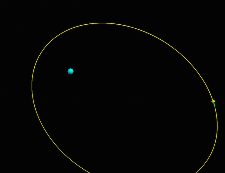
VPython is used to create computational, 3D models of various real world situations in order to better visualize how different equations can manipulate different scenarios. This is very valuable since many of the equations and situations that are coded in vPython are extremely difficult to make a functioning model of in real life.
For instance, the picture below is an example of program that was programmed to show the orbit of a craft around Earth.
This picture shows a graph that tracks
Examples
Simple:
Creating Shapes:
Sphere:
sphere= sphere(pos=vector(-4,-2,5), radius=.4, color=color.red)
Arrow:
bt=arrow(pos=sphere.pos, axis=sphere2.pos-sphere.pos, color=color.cyan)
Vector:
vector=vector(0, 0, 0)
Trail:
trail = curve(color=sphere.color)
trail.append(pos=sphere.pos)
Setting Scene Range:
scene.range=11*sphere.radius
Helix:
spring = helix(pos=ceiling.pos, color=color.cyan, thickness=.003, coils=40, radius=0.015)
Intermediate:
Graphs:
Setup graphing windows:
gdisplay(width=500, height=250, x=600, y=1)
ygraph = gcurve(color=color.yellow)
gdisplay(width=500, height=250, x=600, y=300)
Plotting:
pgraph = gcurve(color=color.blue)
ygraph.plot(pos=(time, Fnet.y))
pgraph.plot(pos=(time, sphere.y))
Difficult:
Using Loops to update Equations:
CONSTANTS:
G = ?
mEarth = ?
mmoon = ?
mcraft = ?
deltat = ?
t = ?
OBJECTS AND INITIAL VALUES:
Earth = sphere(pos=vector(0,0,0), radius=6.4e6, color=color.cyan)
scene.range=11*Earth.radius
Moon = sphere(pos=(4e8, 0, 0), radius=1.75e6, color=color.white)
Add a radius for the spacecraft. It should be BIG, so it can be seen:
craft = sphere(pos=vector(-6.656e7,-3.648e6,0), radius= 10000, color=color.yellow) vcraft = vector(206, 2645,0) pcraft = mcraft*vcraft pArrow=arrow(color=color.green) fArrow=arrow(color=color.cyan) dpArrow=arrow(color=color.red) Fnet_tangent_arrow = arrow(color=color.yellow) Fnet_perp_arrow= arrow(color=color.magenta)
This creates a trail for the spacecraft:
trail = curve(color=craft.color)
And this prevents zooming in or out:
scene.autoscale = 0 pscale=Earth.radius/mag(pcraft) fscale=Earth.radius/((G*mEarth*mcraft)*mag(craft.pos-Earth.pos)**2) dpscale=500*Earth.radius/mag(pcraft) print("p=", pcraft)
CALCULATIONS:
Sets time for loop to run:
while t < 165240: This slows down the animation (runs faster with bigger number):
rate(10000)
    Add statements here for the iterative update of gravitational
   force, momentum, and position.
   r = craft.pos-Earth.pos
   rmag = sqrt(r.x**(2)+r.y**(2)+r.z**(2))
   Fmag= G*mEarth*mcraft/(rmag**2)
   rhat= r/rmag
   rmoon= craft.pos - Moon.pos
   rmoonmag= mag(rmoon)
   rmoonhat= norm(rmoon)
   Fmoonmag= G*mmoon*mcraft/(rmoonmag**2)
   Fmoon= -Fmoonmag*rmoonhat
   p_init= mag(pcraft)
   pcraft_i=pcraft+vector(0,0,0)
   Fearth= -Fmag*rhat
   Fnet= Fearth + Fmoon
   pcraft=Fnet*deltat+pcraft
   p_final=mag(pcraft)
   Fnet_tangent = (p_final-p_init)*norm(pcraft)/deltat
   Fnet_tangent_arrow.pos=craft.pos
   Fnet_tangent_arrow.axis=Fnet_tangent*fscale
   Fnet_perp = Fnet-Fnet_tangent
   Fnet_perp_arrow.pos=craft.pos
   Fnet_perp_arrow.axis=Fnet_perp*fscale
   vcraft=pcraft/mcraft
   craft.pos=vcraft*deltat+craft.pos
   pArrow.pos=craft.pos
   pArrow.axis=pcraft*pscale
   fArrow.pos=craft.pos
   fArrow.axis=Fnet*fscale
   deltap= pcraft-pcraft_i
   dpArrow.pos=craft.pos
   dpArrow.axis=deltap*dpscale
   scene.center=craft.pos
   scene.range=craft.radius*600
  Uncomment these two lines to exit the loop if
  the spacecraft crashes onto the Earth.
   if rmag < Earth.radius:
       break
   trail.append(pos=craft.pos)
   t = t+deltat
Connectedness
vPython codes are very useful in modeling situations that may not be easy to construct models of in real life. The ability to map out a real life scenario in code form and then be able to tweak that code and see how the situation changes is priceless to scientists and students alike. Being able to have a visual in
vPython codes are extremely useful for modeling physics situations. However, the coding skills learned in this class can be applied to almost anything. For example, Aerospace Engineers are becoming increasingly dependent on computer simulations to test ideas before prototyping to reduce costs.
History
A cT language was created in 1997 and was based a language of the PLATO computer-based education system. In 2000 Ruth Chabay, David Scherer, and Bruce Sherwood develop VPython. This form of VPython would be later referred to as "Classic" VPython. From 2002 to 2006 an engineering student named Jonathan Brandmeyer helped make important contributions to VPython 3. As the years went on more and more changes were made in order to make VPython what it is today.
