Acceleration
This page defines and describes acceleration.
The Main Idea
Acceleration, denoted by the symbol [math]\displaystyle{ \vec{a} }[/math], is a vector quantity defined as the rate of change of velocity with respect to time. In calculus terms, it is the time derivative of velocity.
Acceleration is an instantaneous value, so it may change over time.
The most commonly used metric unit for acceleration is the meter per second per second (m/s/s or m/s2).
A Mathematical Model
Instantaneous acceleration is defined as:
[math]\displaystyle{ \vec{a} = \frac{d\vec{v}}{d t} }[/math].
Average Acceleration
Since acceleration is an instantaneous quantity, it can change over time. Over any given time interval, there is an average acceleration value denoted [math]\displaystyle{ \vec{a}_{avg} }[/math]. The average acceleration over an interval of time [math]\displaystyle{ \Delta t }[/math] is given by
[math]\displaystyle{ \vec{a}_{avg} = \frac{\Delta \vec{v}}{\Delta t} }[/math].
Derivative Relationships
Acceleration is the time derivative of velocity, which is in turn the time derivative of position, so acceleration is the second time derivative of position.
Recall that
[math]\displaystyle{ \vec{a}(t) = \frac{d\vec{v}(t)}{dt} }[/math]
and
[math]\displaystyle{ \vec{v}(t) = \frac{d\vec{r}(t)}{dt} }[/math].
Therefore:
[math]\displaystyle{ \vec{a}(t) = \frac{d\vec{v}}{dt} = \frac{d^2\vec{r}}{dt^2} }[/math].
Integral Relationships
The integral of acceleration yields velocity, and the integral of velocity yields position, so the double integral of acceleration yields position.
[math]\displaystyle{ \vec{v}(t) = \int \vec{a}(t) \ dt }[/math]
and
[math]\displaystyle{ \vec{r}(t) = \int \vec{v}(t) \ dt }[/math].
Therefore
[math]\displaystyle{ \vec{r}(t) = \iint \vec{a}(t) \ dt \ dt }[/math].
Kinematic Equations
The kinematic equations can be derived from the derivative and integral relationships between acceleration, velocity, and displacement. For the equations and more information, view the Kinematics page.
Newton's Second Law of Motion
In physics, the acceleration of particles is caused by forces. Newton's Second Law: the Momentum Principle states that
[math]\displaystyle{ \vec{F}_{net} = \frac{d\vec{p}}{dt} }[/math].
From this relation, it can be derived that
[math]\displaystyle{ \vec{F}_{net} = m\vec{a} }[/math]
, or that
[math]\displaystyle{ \vec{a} = \frac{\vec{F}_{net}}{m} }[/math].
This makes sense because acceleration should be directly proportional to force, which causes it, and inversely proportional to mass, which resists it (see Inertia). This equation is often used to find the acceleration of a particle. If that acceleration is constant, kinematic equations are then often used to determine how its position changes over time.
A Graphical Model
Below are some graphs relating velocity and position along one dimension to time as a result of varying types of acceleration. Because of the derivative and integral relationships between position, velocity, and acceleration:
- The slope of a position-vs-time graph at any point in time is the velocity of the particle at that point in time.
- The slope of a velocity-vs-time graph at any point in time is the acceleration of the particle at that point in time.
- The area under a velocity-vs-time graph up to any point in time is the position of the particle at that point in time.
- The area under an acceleration-vs-time graph up to any point in time is the velocity of the particle at that point in time.
Constant Acceleration
When the acceleration of a particle is constant over time, its velocity is changing at a constant rate, and therefore is graphed as a straight line. The acceleration is the slope of the velocity graph; a positive acceleration means the velocity is increasing and should have a positive slope, and a negative acceleration means the velocity is decreasing and has a negative slope.
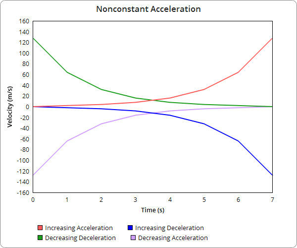
Nonconstant Acceleration
Nonconstant Acceleration is shown with curved lines on velocity over time graphs. Graphs that concave up and are increasing show increasing acceleration, and graphs that concave up and are decreasing show decreasing deceleration. Graphs that concave down and are increasing show decreasing acceleration and graphs that are concave down and decreasing show increasing deceleration.
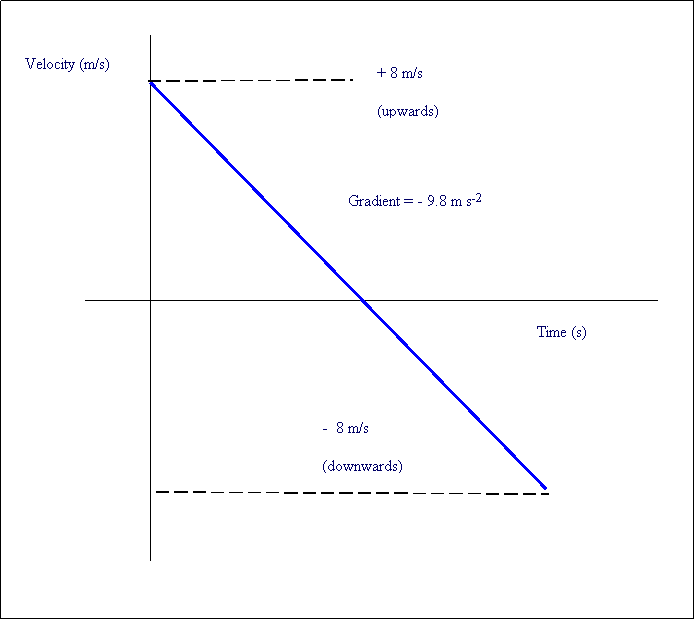
Example
- [Above] Here is a common example showing the velocity of a ball being thrown into the air. Notice that the slope = -9.8 (acceleration due to gravity) and that the graph goes through the x-axis. (The crossover is when the ball is at the highest height and v = 0)
Examples
Here are a couple simple acceleration problems with solutions included:
Question 1

Question:
A motorcycle accelerates uniformly from rest to a speed of 7.10 m/s over a distance of 35.4 m. Determine the acceleration of the motorcycle.
Solution:
Given:
- [math]\displaystyle{ v_i = 0 m/s }[/math]
- [math]\displaystyle{ v_f = 7.10 m/s }[/math]
- [math]\displaystyle{ d = 35.4 m }[/math]
Find:
- [math]\displaystyle{ a = ? }[/math]
Calculations:
- [math]\displaystyle{ v_f^2 = v_i^2 + 2ad }[/math]
- [math]\displaystyle{ 2ad = v_f^2 - v_i^2 }[/math]
- [math]\displaystyle{ a = \frac{v_f^2 - v_i^2}{2*d} }[/math]
- [math]\displaystyle{ a = \frac{(7.10m/s)^2 - (0m/s)^2}{2*35.4m} }[/math]
- [math]\displaystyle{ a = 0.712 m/s^2 }[/math]
Question 2

Question:
A rabbit can jump to a height of 2.62 m. Determine the takeoff speed of the rabbit.
Solution:
Given:
- [math]\displaystyle{ a = -9.8 m/s^2 }[/math]
- [math]\displaystyle{ v_f = 0 m/s }[/math] *Considering the moment of takeoff to maximum height
- [math]\displaystyle{ d = 2.62 m }[/math]
Find:
- [math]\displaystyle{ v_i = ? }[/math]
Calculations:
- [math]\displaystyle{ v_f^2 = v_i^2 + 2ad }[/math]
- [math]\displaystyle{ v_i^2 = 2ad - v_f^2 }[/math]
- [math]\displaystyle{ v_i = \sqrt{2ad - v_f^2} }[/math]
- [math]\displaystyle{ v_i = \sqrt{2*-9.8m/s^2*2.62m - (0m/s)^2} }[/math]
- [math]\displaystyle{ v_i = 7.17 m/s }[/math]
Question 3

Question:
A rock is dropped into a lake and is heard to hit the water 3.41 s after being dropped. Determine the depth of the lake.
Solution:
Given:
- [math]\displaystyle{ a = -9.8 m/s^2 }[/math]
- [math]\displaystyle{ t = 3.41 s }[/math]
- [math]\displaystyle{ v_i = 0 m/s }[/math]
Find:
- [math]\displaystyle{ d = ? }[/math]
Calculations:
- [math]\displaystyle{ d = v_i*t + 0.5*a*t^2 }[/math]
- [math]\displaystyle{ d = (0 m/s)*(3.41 s)+ 0.5*(-9.8 m/s^2)*(3.41 s)^2 }[/math]
- [math]\displaystyle{ d = 0 m + 0.5*(-9.8 m/s^2)*(11.63 s^2) }[/math]
- [math]\displaystyle{ d = -57.0 m }[/math] (57.0 meters deep)
A Computational Model
https://trinket.io/embed/glowscript/569486a2bb
Connectedness
- Acceleration can be applied to many things such as calculating free fall and predicting motion, time and force.
- Acceleration is applied almost everywhere. For example, in biology, it can be used to calculate the growth of plants over time, to predict motion of animals, and even to calculate winds to predict climate changes.
- An interesting industrial application of acceleration is to calculate impacts on cars and to improve quality of manufacturing car safety.
See also
- Kinds of Matter
- Detecting Interactions
- Fundamental Interactions
- System & Surroundings
- Newton's First Law of Motion
- Newton's Second Law of Motion
- Newton's Third Law of Motion
- Gravitational Force
External links
- A physics resource written by experts for an expert audience Physics Portal
- A wiki book on modern physics Modern Physics Wiki
- The MIT open courseware for intro physics MITOCW Wiki
- An online concept map of intro physics HyperPhysics
- Interactive physics simulations PhET
- OpenStax algebra based intro physics textbook College Physics
- The Open Source Physics project is a collection of online physics resources OSP
- A resource guide compiled by the AAPT for educators ComPADRE
References
- Chabay, Ruth W., and Bruce A. Sherwood. Matter & Interactions. 4th ed. Hoboken, NJ: John Wiley & Sons, 2015. Print.
- "Acceleration as derivative of velocity along trajectory" by Fred the OysteriThe source code of this SVG is valid.This vector graphics image was created with Adobe Illustrator.. Licensed under GFDL via Commons - https://commons.wikimedia.org/wiki/File:Acceleration_as_derivative_of_velocity_along_trajectory.svg#/media/File:Acceleration_as_derivative_of_velocity_along_trajectory.svg
- "Staw naturalny" by Mohylek - Own work. Licensed under GFDL via Commons - https://commons.wikimedia.org/wiki/File:Staw_naturalny.JPG#/media/File:Staw_naturalny.JPG
- "Triumph T 110 650 cc 1954" by Yesterdays Antique Motorcycles - http://www.yesterdays.nl/images/Triumph%201954%20T110-1.jpg. Licensed under CC BY-SA 3.0 via Commons - https://commons.wikimedia.org/wiki/File:Triumph_T_110_650_cc_1954.jpg#/media/File:Triumph_T_110_650_cc_1954.jpg
- "Velocity-Time Graphs" by Keith Gibbs. http://www.schoolphysics.co.uk/age14-16/Mechanics/Motion/text/Velocity_time_graphs/index.html
- "Rabbit in montana" by Larry D. Moore. Licensed under CC BY-SA 3.0 via Commons - https://commons.wikimedia.org/wiki/File:Rabbit_in_montana.jpg#/media/File:Rabbit_in_montana.jpg


