Python Syntax
Edited by Zach Sanchez - Fall 2017 (in progress)
The Main Idea
VPython is an extension of the Python programming language that contains a 3D graphics module called Visual, which allows users to create simple simulations of physics problems. Its primary use is for educational purposes, although it has been used in research before in the past. We will use VPython on occasion to aid us in visualizing and experimenting with the ideas that we learn in this course.
Downloading vPython
In all cases you will need to have Python 2.7.9 installed. Future versions may also work, but be warned that it may cause VPython to behave erratically.
Note for Linux: You can only install Classic VPython, which is no longer supported and may be missing some features and bug fixes that are present in the current version of VPython.
Alternatively, you can use GlowScript, a virtual environment that allows you to execute VPython code in your browser. You can create an account at http://www.glowscript.org/.
Python Basics
It's always helpful to have a background knowledge of Python, however basic, before proceeding with the applications more relevant to this course.
   # Comments start with a number symbol. Use these liberally in order to keep track of the changes you make/the code you write.
   # We're always going to start our programs with the following headers to ensure that math works correctly.
   from__future__ import division
   from visual import*
   # Math works as you would expect.
   1 + 1  # -> 2
   2 - 1  # -> 1
   3 * 2  # -> 6
   8 / 4  # -> 4
   (1 + 3) * 2  # -> 8
   1 + (3 * 2)  # -> 7
   # That is, until you need to do an exponent. But you shouldn't encounter anything much weirder than that math-wise.
   2 ** 3  # -> 8
   # However, these math operations are useless if we don't store the values anywhere.
   x = 1 + 1
   # Now if you try to access x in the future, it will have the value of '2'.
   # You can print your variables like this:
   print(x)
   # You can also add in some text with them like this:
   print("The value of x is ", x)
   # Sometimes we only want to execute something based on a certain condition.
   if x == 2:
       y = 3
   # The '==' means that you're directly comparing two values. If they're equal, whatever is on the inside of the if-statement will be executed.
   # Now is a good time to note that whitespace is very important in Python. 'y = 3' will always execute if it isn't tabbed, so even if x is equal to 7, y will still become 3.
   # If you ever see me use whitespace in this tutorial, make sure you do as well.
   # Some other useful comparators: != (not equal), >, >= (greater than or equal to), <, <= (less than or equal to), 'and', 'or', 'not'
   # You can add onto the above if-statement by tacking on:
   elif x == 3:
       y = 4
   else:
       y = 5
   # With elif meaning "else if" for a second possible condition, and "else" for something that you want to execute if none of the earlier conditions are met.
   # You can also have a loop that executes code for a certain amount of time or based on a certain condition.
   while x < 5:
       print("x is ", x)
       x = x + 1
   # This will output the value of x up until it reaches 4.
Thus concludes our very, very brief foray into Python. That was simply the bare minimum required to understand what will be needed for this class. More concepts will be introduced as needed, whether that be in this tutorial or in a lab. For a more complete understanding of Python, you can look up other Python tutorials elsewhere on the Internet.
Mathematical Model
Vpython can compute any equation, but some that may be most helpful and most useful for Physics can be found below. (Keep in mind you can alter these numbers to be whatever you need, these are just to provide an example):
To update momentum:
pf = pi + Fnet*deltat
To update position:
objectf.pos = objecti.pos + (pcart/mcart)*deltat
To create a vector:
vector(0,0,0) -- fill in with whatever numbers the vector should be
Gravitational Force:
   # Constants
   G = 6.7e-11
   mEarth = 6e24
   mcraft = 15e3
   deltat = 60
   t = 0
Finds the change in position:
   r=craft.pos-Earth.pos
   m=mcraft
To find the magnitude of the change in position:
rmag= mag(r)
To calculate the new magnitude of gravitational force:
Fmag=(G*mcraft*mEarth)/(rmag**2)
To calculate the direction of the change in position:
rhat=r/rmag
To calculate net force:
Fnet=-Fmag*rhat
To calculate spring force:
   L0 = 0.3
   Lvec = ball.pos - ceiling.pos
   Lhat = norm(Lvec)
   Lmag = mag(Lvec)
   Fspr = (-ks)*(Lmag - L0)*(Lhat)
To calculate kinetic energy:
Kinetic = (1/2)*(mball*(vel**2))
To create a graph:
   gdisplay(width=500, height=250, x=600, y=1)
   ygraph= gcurve(color=color.cyan)
To add plots to the graph:
ygraph.plot(pos=(t, fnet.y))
Computational Model
VPython is used to create computational, 3D models of various real world situations in order to better visualize how different equations can manipulate different scenarios. This is very valuable since many of the equations and situations that are coded in vPython are extremely difficult to make a functioning model of in real life.
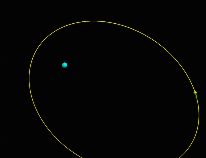
For instance, the picture below is an example of program that was programmed to show the orbit of a craft around Earth.
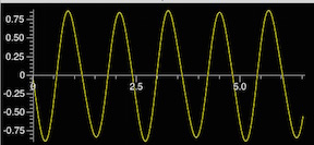
This picture shows a graph that tracks.

Examples
Simple:
Creating Shapes:
Sphere:
sphere= sphere(pos=vector(-4,-2,5), radius=.4, color=color.red)
Arrow:
bt=arrow(pos=sphere.pos, axis=sphere2.pos-sphere.pos, color=color.cyan)
Vector:
vector=vector(0, 0, 0)
Trail:
   trail = curve(color=sphere.color)
   trail.append(pos=sphere.pos)
Setting Scene Range:
scene.range=11*sphere.radius
Helix:
spring = helix(pos=ceiling.pos, color=color.cyan, thickness=.003, coils=40, radius=0.015)
Intermediate:
Graphs:
Setup graphing windows:
   gdisplay(width=500, height=250, x=600, y=1)
   ygraph = gcurve(color=color.yellow)
   gdisplay(width=500, height=250, x=600, y=300)
Plotting:
   pgraph = gcurve(color=color.blue)
   ygraph.plot(pos=(time, Fnet.y))
   pgraph.plot(pos=(time, sphere.y))
Difficult:
Using Loops to update Equations:
Constants:
G = ?
mEarth = ?
mmoon = ?
mcraft = ?
deltat = ?
t = ?
Objects and initial values:
   Earth = sphere(pos=vector(0,0,0), radius=6.4e6, color=color.cyan)
   scene.range=11*Earth.radius
   Moon = sphere(pos=(4e8, 0, 0), radius=1.75e6, color=color.white)
Add a radius for the spacecraft. It should be BIG, so it can be seen:
   craft = sphere(pos=vector(-6.656e7,-3.648e6,0), radius= 10000, color=color.yellow)
   vcraft = vector(206, 2645,0)
   pcraft = mcraft*vcraft
   pArrow=arrow(color=color.green)
   fArrow=arrow(color=color.cyan)
   dpArrow=arrow(color=color.red)
   Fnet_tangent_arrow = arrow(color=color.yellow)
   Fnet_perp_arrow= arrow(color=color.magenta)
This creates a trail for the spacecraft:
trail = curve(color=craft.color)
And this prevents zooming in or out:
   scene.autoscale = 0
   pscale=Earth.radius/mag(pcraft)
   fscale=Earth.radius/((G*mEarth*mcraft)*mag(craft.pos-Earth.pos)**2)
   dpscale=500*Earth.radius/mag(pcraft)
   print("p=", pcraft)
Calculations:
Sets time for loop to run:
while t < 165240:
This slows down the animation (runs faster with bigger number):
rate(10000)
Add statements here for the iterative update of gravitational force, momentum, and position.
   r = craft.pos-Earth.pos
   rmag = sqrt(r.x**(2)+r.y**(2)+r.z**(2))
   Fmag= G*mEarth*mcraft/(rmag**2)
   rhat= r/rmag
   rmoon= craft.pos - Moon.pos
   rmoonmag= mag(rmoon)
   rmoonhat= norm(rmoon)
   Fmoonmag= G*mmoon*mcraft/(rmoonmag**2)
   Fmoon= -Fmoonmag*rmoonhat
   p_init= mag(pcraft)
   pcraft_i=pcraft+vector(0,0,0)
   Fearth= -Fmag*rhat
   Fnet= Fearth + Fmoon
   pcraft=Fnet*deltat+pcraft
   p_final=mag(pcraft)
   Fnet_tangent = (p_final-p_init)*norm(pcraft)/deltat
   Fnet_tangent_arrow.pos=craft.pos
   Fnet_tangent_arrow.axis=Fnet_tangent*fscale
   Fnet_perp = Fnet-Fnet_tangent
   Fnet_perp_arrow.pos=craft.pos
   Fnet_perp_arrow.axis=Fnet_perp*fscale
   vcraft=pcraft/mcraft
   craft.pos=vcraft*deltat+craft.pos
   pArrow.pos=craft.pos
   pArrow.axis=pcraft*pscale
   fArrow.pos=craft.pos
   fArrow.axis=Fnet*fscale
   deltap= pcraft-pcraft_i
   dpArrow.pos=craft.pos
   dpArrow.axis=deltap*dpscale
   scene.center=craft.pos
   scene.range=craft.radius*600

  Uncomment these two lines to exit the loop if
  the spacecraft crashes onto the Earth.
   if rmag < Earth.radius:
       break
   trail.append(pos=craft.pos)
   t = t+deltat
