Main Page: Difference between revisions
LukasYoder (talk | contribs) Undo revision 32772 by LukasYoder (talk) |
LukasYoder (talk | contribs) Undo revision 32770 by LukasYoder (talk) |
||
| Line 504: | Line 504: | ||
===Week 4=== | ===Week 4=== | ||
<div class="toccolours mw-collapsible mw-collapsed"> | <div class="toccolours mw-collapsible mw-collapsed"> | ||
====Field of a Charged | =Field of a Charged Rod= | ||
'''This entire page and all its contents were created by Lukas Yoder, PHYS 2212 Class of Fall 2018''' | |||
=== The Main Idea === | |||
Previously, we've learned about the electric field of a point particle. Often, when analyzing physical systems, it is the case that we're unable to analyze each individual particle that composes an object and need to therefore generalize collections of particles into shapes (in this case, a rod) whereby the mathematics corresponding to electric field calculations can be simplified. This can essentially be done by adding up the contributions to the electric field made by parts of an object, approximating each part of an object as a point charge. | |||
=== The System in Question === | |||
As discussed in the previous section, we're considering a system | |||
abstracted from the particle model we're familiar with, therefore we will | |||
make the generalization that our rod of length L has a total charge of | |||
quantity Q. For this generalization, we will need to assume that the rod | |||
is so thin that we can ignore its thickness. | |||
[[Image:LukasYoder01.jpg|200px|center]] | |||
Since the electric field produced by a charge at any given location is | |||
proportional to the distance from the charge to that location, we will | |||
need to relate the observation location to the source of the charge, which | |||
we will consider the origin of the rod. To do that, we will need to divide | |||
the rod into pieces of length \delta y each containing a charge \delta Q. | |||
In the image below, you can see what this looks like and the relation that | |||
can be found between the observation location and the source, forming the | |||
distance vector \vect{r}. | |||
[[Image:LukasYoder02.jpg|400px|center]] | |||
By the pythagorean theorem, we can find the vector \vect{r} as follows: | |||
[[Image:LukasYoder03.jpg|400px|center]] | |||
And to find the unit vector in the direction of \vect{r}, \hat{r}, we do as | |||
follows: | |||
[[Image:LukasYoder04.jpg|400px|center]] | |||
=== Finding the Contribution of Each Piece to the Electric Field === | |||
Now that we've set up a model for the system, with the rod broken down | |||
into pieces, we can find the contribution of each piece to the electric | |||
field of the system. We will start from the electric field equation you | |||
learned for a point particle but plug in the parameters for the rod system | |||
into the equation. | |||
[[Image:LukasYoder05.jpg|400px|center]] | |||
By mathematically simplifying, we then get the following equation: | |||
[[Image:LukasYoder06.jpg|400px|center]] | |||
=== Finding the Net Contribution of all Pieces === | |||
In the previous section, we found out the contribution to the electric | |||
field at a given location of only one of the pieces constituting the rod. | |||
In order to figure out the net field at any particular location, we need | |||
to add up the electric fields produced by individual pieces along the | |||
length of the rod. | |||
We will switch from vector notation for the electric field to the scalar | |||
notation for the x- and y-components. (From the vector in the equation | |||
above, we can see that the z-component of the electric field at any point | |||
is always 0.) The x-component of the electric | |||
field is the sum of the x-components of every \delta{y} along the rod, and | |||
the y-component of the electric field is the sum of the y-components of | |||
every \delta{y} along the rod. We can show this mathematically: | |||
[[Image:LukasYoder07.jpg|400px|center]] | |||
To make use of this relation, because we don't know \delta{Q}, we need to | |||
relate it to parameters that we already know about the rod system we're | |||
analyzing. We can express \delta{Q} as the charge density of the rod | |||
(which is Q/L) times the \delta{y} we've chosen for the system. Thus, | |||
[[Image:LukasYoder08.jpg|200px|center]] | |||
By plugging the above equation into our equations for the x- and | |||
y-components of the electric field at a point, we can find the electric | |||
field at any point in the system. This technique is called numerical | |||
integration and is typically done by computers because the computational | |||
complexity is dependant upon the size of \delta{y} with respect to L. | |||
=== Simplifying === | |||
Using calculus, we can simplify a lot of the math required to compute the | |||
electric field at any given point. Notationally, all we're doing is switching from the | |||
discretely-sized \delta{y} to \textit{dy} and from the sigma notation to | |||
an integral starting from -L/2 (the lower end of the rod) and ending at | |||
L/2 (the upper end of the rod) as follows: | |||
[[Image:LukasYoder09.jpg|400px|center]] | |||
[[Image:LukasYoder10.jpg|400px|center]] | |||
By evaluating the integral, we can determine that the x-component of the | |||
electric field at any point is: | |||
[[Image:LukasYoder11.jpg|400px|center]] | |||
Without evaluating the integral for the y-component of the electric field, | |||
we can use symmetry to determine that the y-component of the electric | |||
field at any given point is 0. Let's consider the contributions to the | |||
electric field from the top and bottom halves of the rod at any | |||
observation point. | |||
[[Image:LukasYoder12.jpg|200px|center]] | |||
Since the y-components of E_top and E_bottom are of equal magnitude and | |||
opposite direction, they cancel each other out, and therefore the | |||
y-component of teh electric field at any given point due to the rod is 0. | |||
[[Image:LukasYoder13.jpg|200px|center]] | |||
Finally, because the rod is round and can be rotated, as a convenience, | |||
we'll use d (distance from the rod) as opposed to x (distance along the | |||
x-direction) to refer to the electric field. | |||
Thus we can simplify electric field calculations for a rod into a form | |||
that we can readily use: | |||
[[Image:LukasYoder14.jpg|400px|center]] | |||
=== Further Simplification === | |||
By noting the contributions of each variable to the equation for the | |||
electric field, we can make approximations to simplify our math by simply | |||
declaring one variable as insignificant. | |||
For example, if we have a system in which the length of a rod is much | |||
greater than the magnitude of the distance from the rod (denoted L>>d), we | |||
can neglect some of the instances in which d is taken into account as | |||
follows: | |||
[[Image:LukasYoder15.jpg|400px|center]] | |||
=== Finding the Electric Field from a Rod with Code === | |||
Here is some code that you can run which shows the electric field vector | |||
at a given distance from the rod along its length. The rod is shown as a | |||
series of green balls to help emphasize that when using the numerical | |||
integrations mentioned on this page, you are measuring the field produced | |||
by discrete parts of the rod being analyzed. | |||
Notice the edge-effects of the electric field of the rod. For reasons | |||
discussed above, if we used the long rod approximation (L>>d), these | |||
effects would be negligible. | |||
[http://www.glowscript.org/#/user/yoderlukas/folder/Public/program/ElectricFieldAlongRodLength Click Here to Run the Code] | |||
===Week 5=== | |||
<div class="toccolours mw-collapsible mw-collapsed"> | |||
====Potential energy==== | |||
'''Written by Lukas Yoder, PHYS 2212 Class of Fall 2018''' | |||
<div class="mw-collapsible-content"> | |||
*[[Potential Energy]] | |||
== The Main Idea == | |||
Potential energy is the energy that an object has because of its characteristics relative to other objects within the universe. In Physics 1 | |||
</div> | |||
</div> | |||
<div class="toccolours mw-collapsible mw-collapsed"> | |||
====Electric potential==== | |||
<div class="mw-collapsible-content"> | |||
*[[Electric Potential]] | |||
*[[Path Independence of Electric Potential]] | |||
*[[Potential Difference Path Independence, claimed by Aditya Mohile]] | |||
*[[Potential Difference in a Uniform Field]] | |||
*[[Potential Difference of Point Charge in a Non-Uniform Field]] | |||
</div> | |||
</div> | |||
<div class="toccolours mw-collapsible mw-collapsed"> | |||
====Sign of a potential difference==== | |||
<div class="mw-collapsible-content"> | |||
*[[Sign of a Potential Difference]] | |||
</div> | |||
</div> | |||
<div class="toccolours mw-collapsible mw-collapsed"> | |||
====Potential at a single location==== | |||
<div class="mw-collapsible-content"> | |||
*[[Electric Potential]] | |||
*[[Potential Difference at One Location]] | |||
</div> | |||
</div> | |||
<div class="toccolours mw-collapsible mw-collapsed"> | |||
====Path independence and round trip potential==== | |||
<div class="mw-collapsible-content"> | |||
*[[Path Independence of Electric Potential]] | |||
*[[Potential Difference Path Independence, claimed by Aditya Mohile]] | |||
</div> | |||
</div> | |||
===Week 6=== | |||
<div class="toccolours mw-collapsible mw-collapsed"> | |||
====Electric field and potential in an insulator==== | |||
<div class="mw-collapsible-content"> | |||
*[[Potential Difference in an Insulator]] | |||
*[[Electric Field in an Insulator]] | |||
</div> | |||
</div> | |||
<div class="toccolours mw-collapsible mw-collapsed"> | |||
====Moving charges in a magnetic field==== | |||
<div class="mw-collapsible-content"> | |||
*[[Magnetic Field]] | |||
*[[Magnetic Force]] | |||
*[[Lorentz Force]] | |||
</div> | |||
</div> | |||
<div class="toccolours mw-collapsible mw-collapsed"> | |||
====Biot-Savart Law==== | |||
<div class="mw-collapsible-content"> | |||
*[[Biot-Savart Law]] | |||
*[[Biot-Savart Law for Currents]] | |||
</div> | |||
</div> | |||
<div class="toccolours mw-collapsible mw-collapsed"> | |||
====Moving charges, electron current, and conventional current==== | |||
<div class="mw-collapsible-content"> | |||
*[[Moving Point Charge]] | |||
*[[Current]] | |||
</div> | |||
</div> | |||
===Week 7=== | |||
<div class="toccolours mw-collapsible mw-collapsed"> | |||
====Magnetic field of a wire==== | |||
<div class="mw-collapsible-content"> | |||
*[[Magnetic Field of a Long Straight Wire]] | |||
</div> | |||
</div> | |||
<div class="toccolours mw-collapsible mw-collapsed"> | |||
====Magnetic field of a current-carrying loop==== | |||
<div class="mw-collapsible-content"> | |||
*[[Magnetic Field of a Loop]] | |||
</div> | |||
</div> | |||
<div class="toccolours mw-collapsible mw-collapsed"> | |||
====Magnetic field of a Charged Disk==== | |||
<div class="mw-collapsible-content"> | |||
*[[Magnetic Field of a Disk]] | |||
</div> | |||
</div> | |||
<div class="toccolours mw-collapsible mw-collapsed"> | |||
====Magnetic dipoles==== | |||
<div class="mw-collapsible-content"> | |||
*[[Magnetic Dipole Moment]] | |||
*[[Bar Magnet]] | |||
</div> | |||
</div> | |||
<div class="toccolours mw-collapsible mw-collapsed"> | |||
====Atomic structure of magnets==== | |||
<div class="mw-collapsible-content"> | |||
*[[Atomic Structure of Magnets]] | |||
</div> | |||
</div> | |||
===Week 8=== | |||
<div class="toccolours mw-collapsible mw-collapsed"> | |||
====Steady state current==== | |||
<div class="mw-collapsible-content"> | |||
*[[Steady State]] | |||
*[[Non Steady State]] | |||
</div> | |||
</div> | |||
<div class="toccolours mw-collapsible mw-collapsed"> | |||
====Kirchoff's Laws==== | |||
<div class="mw-collapsible-content"> | |||
*[[Kirchoff's Laws]] | |||
</div> | |||
</div> | |||
<div class="toccolours mw-collapsible mw-collapsed"> | |||
====Electric fields and energy in circuits==== | |||
<div class="mw-collapsible-content"> | |||
*[[Series circuit]] | |||
*[[Node Rule]] | |||
*[[Loop Rule]] | |||
*[[Electric Potential Difference]] | |||
</div> | |||
</div> | |||
<div class="toccolours mw-collapsible mw-collapsed"> | |||
====Macroscopic analysis of circuits==== | |||
<div class="mw-collapsible-content"> | |||
*[[Series Circuits]] | |||
*[[Parallel Circuits]] | |||
*[[Parallel Circuits vs. Series Circuits*]] | |||
*[[Loop Rule]] | |||
*[[Node Rule]] | |||
*[[Fundamentals of Resistance]] | |||
*[[Problem Solving]] | |||
</div> | |||
</div> | |||
===Week 9=== | |||
<div class="toccolours mw-collapsible mw-collapsed"> | |||
====Electric field and potential in circuits with capacitors==== | |||
<div class="mw-collapsible-content"> | |||
*[[Charging and Discharging a Capacitor]] | |||
*[[RC Circuit]] | |||
*[[R Circuit]] | |||
*[[AC and DC]] | |||
</div> | |||
</div> | |||
<div class="toccolours mw-collapsible mw-collapsed"> | |||
====Magnetic forces on charges and currents==== | |||
<div class="mw-collapsible-content"> | |||
*[[Magnetic Force]] | |||
*[[Lorentz Force]] | |||
*[[Motors and Generators]] | |||
*[[Applying Magnetic Force to Currents]] | |||
*[[Magnetic Force in a Moving Reference Frame]] | |||
*[[Right-Hand Rule]] | |||
*[[Analysis of Railgun vs Coil gun technologies]] | |||
</div> | |||
</div> | |||
<div class="toccolours mw-collapsible mw-collapsed"> | |||
====Electric and magnetic forces==== | |||
<div class="mw-collapsible-content"> | |||
*[[Electric Force]] | |||
*[[Magnetic Force]] | |||
*[[Lorentz Force]] | |||
*[[VPython Modelling of Electric and Magnetic Forces]] | |||
</div> | |||
</div> | |||
<div class="toccolours mw-collapsible mw-collapsed"> | |||
====Velocity selector==== | |||
<div class="mw-collapsible-content"> | |||
*[[Lorentz Force]] | |||
*[[Combining Electric and Magnetic Forces]] | |||
</div> | |||
</div> | |||
===Week 10=== | |||
<div class="toccolours mw-collapsible mw-collapsed"> | |||
====Hall Effect==== | |||
<div class="mw-collapsible-content"> | |||
*[[Hall Effect]] | |||
*[[Right-Hand Rule]] | |||
*[[Motional Emf]] | |||
*[[Magnetic Force]] | |||
*[[Magnetic Torque]] | |||
</div> | |||
</div> | |||
<div class="toccolours mw-collapsible mw-collapsed"> | |||
====Motional EMF==== | |||
<div class="mw-collapsible-content"> | |||
*[[Motional Emf]] | |||
*[[Motional Emf using Faraday's Law]] | |||
</div> | |||
</div> | |||
<div class="toccolours mw-collapsible mw-collapsed"> | |||
====Magnetic force==== | |||
<div class="mw-collapsible-content"> | |||
*[[Magnetic Force]] | |||
*[[Lorentz Force]] | |||
</div> | |||
</div> | |||
<div class="toccolours mw-collapsible mw-collapsed"> | |||
====Magnetic torque==== | |||
<div class="mw-collapsible-content"> | |||
*[[Magnetic Torque]] | |||
*[[Right-Hand Rule]] | |||
</div> | |||
</div> | |||
===Week 12=== | |||
<div class="toccolours mw-collapsible mw-collapsed"> | |||
====Gauss's Law==== | |||
<div class="mw-collapsible-content"> | |||
*[[Gauss's Flux Theorem]] | |||
*[[Gauss's Law]] | |||
*[[Magnetic Flux]] | |||
</div> | |||
</div> | |||
<div class="toccolours mw-collapsible mw-collapsed"> | |||
====Ampere's Law==== | |||
<div class="mw-collapsible-content"> | |||
*[[Ampere's Law]] | |||
*[[Ampere-Maxwell Law]] | |||
*[[Magnetic Field of Coaxial Cable Using Ampere's Law]] | |||
*[[Magnetic Field of a Long Thick Wire Using Ampere's Law]] | |||
*[[Magnetic Field of a Toroid Using Ampere's Law]] | |||
*[[Magnetic Field of a Solenoid Using Ampere's Law]] | |||
*[[The Differential Form of Ampere's Law]] | |||
</div> | |||
</div> | |||
===Week 13=== | |||
<div class="toccolours mw-collapsible mw-collapsed"> | |||
====Semiconductors==== | |||
<div class="mw-collapsible-content"> | |||
*[[Semiconductor Devices]] | |||
</div> | |||
</div> | |||
<div class="toccolours mw-collapsible mw-collapsed"> | |||
====Faraday's Law==== | |||
<div class="mw-collapsible-content"> | |||
*[[Faraday's Law]] | |||
*[[Motional Emf using Faraday's Law]] | |||
*[[Lenz's Law]] | |||
</div> | |||
</div> | |||
<div class="toccolours mw-collapsible mw-collapsed"> | |||
====Maxwell's equations==== | |||
<div class="mw-collapsible-content"> | |||
*[[Gauss's Law]] | |||
*[[Magnetic Flux]] | |||
*[[Ampere's Law]] | |||
*[[Faraday's Law]] | |||
*[[Maxwell's Electromagnetic Theory]] | |||
</div> | |||
</div> | |||
===Week 14=== | |||
<div class="toccolours mw-collapsible mw-collapsed"> | |||
====Circuits revisited==== | |||
<div class="mw-collapsible-content"> | |||
</div> | |||
</div> | |||
<div class="toccolours mw-collapsible mw-collapsed"> | |||
====Inductors==== | |||
<div class="mw-collapsible-content"> | |||
*[[Inductors]] | |||
*[[Current in an LC Circuit]] | |||
*[[Current in an RL Circuit]] | |||
</div> | |||
</div> | |||
===Week 15=== | |||
<div class="toccolours mw-collapsible mw-collapsed"> | |||
==== Electromagnetic Radiation ==== | |||
<div class="mw-collapsible-content"> | |||
*[[Electromagnetic Radiation]] | |||
</div> | |||
</div> | |||
<div class="toccolours mw-collapsible mw-collapsed"> | |||
====Sparks in the air==== | |||
<div class="mw-collapsible-content"> | |||
*[[Sparks in Air]] | |||
*[[Spark Plugs]] | |||
</div> | |||
</div> | |||
<div class="toccolours mw-collapsible mw-collapsed"> | |||
====Superconductors==== | |||
<div class="mw-collapsible-content"> | |||
*[[Superconducters]] | |||
*[[Superconductors]] | |||
*[[Meissner effect]] | |||
</div> | |||
</div> | |||
</div> | |||
<div style="float:left; width:30%; padding:1%;"> | |||
==Physics 3== | |||
===Week 1=== | |||
<div class="toccolours mw-collapsible mw-collapsed"> | |||
====Classical Physics==== | |||
<div class="mw-collapsible-content"> | |||
</div> | |||
</div> | |||
===Week 2=== | |||
<div class="toccolours mw-collapsible mw-collapsed"> | |||
====Special Relativity==== | |||
<div class="mw-collapsible-content"> | |||
*[[Frame of Reference]] | |||
*[[Einstein's Theory of Special Relativity]] | |||
*[[Time Dilation]] | |||
*[[Einstein's Theory of General Relativity]] | |||
*[[Albert A. Micheleson & Edward W. Morley]] | |||
*[[Magnetic Force in a Moving Reference Frame]] | |||
</div> | |||
</div> | |||
===Week 3=== | |||
<div class="toccolours mw-collapsible mw-collapsed"> | |||
====Photons==== | |||
<div class="mw-collapsible-content"> | |||
*[[Spontaneous Photon Emission]] | |||
*[[Light Scattering: Why is the Sky Blue]] | |||
*[[Lasers]] | |||
*[[Electronic Energy Levels and Photons]] | |||
*[[Quantum Properties of Light]] | |||
</div> | |||
</div> | |||
===Week 4=== | |||
<div class="toccolours mw-collapsible mw-collapsed"> | |||
====Matter Waves==== | |||
<div class="mw-collapsible-content"> | |||
*[[Wave-Particle Duality]] | |||
</div> | |||
</div> | |||
===Week 5=== | |||
<div class="toccolours mw-collapsible mw-collapsed"> | |||
====Wave Mechanics==== | |||
<div class="mw-collapsible-content"> | |||
*[[Standing Waves]] | |||
*[[Wavelength]] | |||
*[[Wavelength and Frequency]] | |||
*[[Mechanical Waves]] | |||
*[[Transverse and Longitudinal Waves]] | |||
</div> | |||
</div> | |||
===Week 6=== | |||
<div class="toccolours mw-collapsible mw-collapsed"> | |||
====Rutherford-Bohr Model==== | |||
<div class="mw-collapsible-content"> | |||
*[[Rutherford Experiment and Atomic Collisions]] | |||
*[[Bohr Model]] | |||
*[[Quantized energy levels]] | |||
*[[Energy graphs and the Bohr model]] | |||
</div> | |||
</div> | |||
===Week 7=== | |||
<div class="toccolours mw-collapsible mw-collapsed"> | |||
====The Hydrogen Atom==== | |||
<div class="mw-collapsible-content"> | |||
*[[Quantum Theory]] | |||
*[[Atomic Theory]] | |||
</div> | |||
</div> | |||
===Week 8=== | |||
<div class="toccolours mw-collapsible mw-collapsed"> | |||
====Many-Electron Atoms==== | |||
<div class="mw-collapsible-content"> | |||
*[[Quantum Theory]] | |||
*[[Atomic Theory]] | |||
*[[Pauli exclusion principle]] | |||
</div> | |||
</div> | |||
===Week 9=== | |||
<div class="toccolours mw-collapsible mw-collapsed"> | |||
====Molecules==== | |||
<div class="mw-collapsible-content"> | |||
</div> | |||
</div> | |||
===Week 10=== | |||
<div class="toccolours mw-collapsible mw-collapsed"> | |||
====Statistical Physics==== | |||
<div class="mw-collapsible-content"> | |||
</div> | |||
</div> | |||
===Week 11=== | |||
<div class="toccolours mw-collapsible mw-collapsed"> | |||
====Condensed Matter Physics==== | |||
<div class="mw-collapsible-content"> | |||
</div> | |||
</div> | |||
===Week 12=== | |||
<div class="toccolours mw-collapsible mw-collapsed"> | |||
====The Nucleus==== | |||
<div class="mw-collapsible-content"> | |||
*[[Nucleus]] | |||
</div> | |||
</div> | |||
===Week 13=== | |||
<div class="toccolours mw-collapsible mw-collapsed"> | |||
====Nuclear Physics==== | |||
<div class="mw-collapsible-content"> | |||
*[[Nuclear Fission]] | |||
*[[Nuclear Energy from Fission and Fusion]] | |||
</div> | |||
</div> | |||
===Week 14=== | |||
<div class="toccolours mw-collapsible mw-collapsed"> | |||
====Particle Physics==== | |||
<div class="mw-collapsible-content"> | |||
*[[Elementary Particles and Particle Physics Theory]] | |||
*[[String Theory]] | |||
</div> | |||
</div> | |||
</div> | |||
Revision as of 01:14, 26 November 2018
Georgia Tech Student Wiki for Introductory Physics.
This resource was created so that students can contribute and curate content to help those with limited or no access to a textbook. When reading this website, please correct any errors you may come across. If you read something that isn't clear, please consider revising it for future students!
Looking to make a contribution?
- Pick one of the topics from intro physics listed below
- Add content to that topic or improve the quality of what is already there.
- Need to make a new topic? Edit this page and add it to the list under the appropriate category. Then copy and paste the default Template into your new page and start editing.
Please remember that this is not a textbook and you are not limited to expressing your ideas with only text and equations. Whenever possible embed: pictures, videos, diagrams, simulations, computational models (e.g. Glowscript), and whatever content you think makes learning physics easier for other students.
Source Material
All of the content added to this resource must be in the public domain or similar free resource. If you are unsure about a source, contact the original author for permission. That said, there is a surprisingly large amount of introductory physics content scattered across the web. Here is an incomplete list of intro physics resources (please update as needed).
- A physics resource written by experts for an expert audience Physics Portal
- A wiki written for students by a physics expert MSU Physics Wiki
- A wiki book on modern physics Modern Physics Wiki
- The MIT open courseware for intro physics MITOCW Wiki
- An online concept map of intro physics HyperPhysics
- Interactive physics simulations PhET
- OpenStax intro physics textbooks: Vol1, Vol2, Vol3
- The Open Source Physics project is a collection of online physics resources OSP
- A resource guide compiled by the AAPT for educators ComPADRE
- The Feynman lectures on physics are free to read Feynman
- Final Study Guide for Modern Physics II created by a lab TA Modern Physics II Final Study Guide
Resources
- Commonly used wiki commands Wiki Cheatsheet
- A guide to representing equations in math mode Wiki Math Mode
- A page to keep track of all the physics Constants
- A page for review of Vectors and vector operations
- A listing of Notable Scientist with links to their individual pages
Physics 1
Week 1
Help with VPython
VPython
Interactions
Velocity and Momentum
Week 2
Momentum and the Momentum Principle
Iterative Prediction with a Constant Force
Week 3
Analytic Prediction with a Constant Force
Iterative Prediction with a Varying Force
Week 4
Fundamental Interactions
Week 5
Conservation of Momentum
Properties of Matter
Week 6
Identifying Forces
Week 7
Energy Principle
Week 8
Work by Non-Constant Forces
Potential Energy
Week 9
Multiparticle Systems
Week 10
Choice of System
Thermal Energy, Dissipation, and Transfer of Energy
- Thermal Energy
- Specific Heat
- Heat Capacity
- Calorific Value(Heat of combustion)
- Specific Heat Capacity
- First Law of Thermodynamics
- Second Law of Thermodynamics and Entropy
- Temperature
- Predicting Change
- Energy Transfer due to a Temperature Difference
- Transformation of Energy
- The Maxwell-Boltzmann Distribution
- Air Resistance
Rotational and Vibrational Energy
Week 11
Different Models of a System
Models of Friction
Week 12
Collisions
Week 13
Rotations
Angular Momentum
- Total Angular Momentum
- Translational Angular Momentum
- Rotational Angular Momentum
- The Angular Momentum Principle
- Angular Momentum Compared to Linear Momentum
- Angular Impulse
- Predicting the Position of a Rotating System
- Angular Momentum of Multiparticle Systems
- The Moments of Inertia
- Moment of Inertia for a cylinder
- Right Hand Rule
Week 14
Analyzing Motion with and without Torque
Week 15
Introduction to Quantum Concepts
Physics 2
Week 1
3D Vectors
Electric field
Electric force
Electric field of a point particle
Superposition
Dipoles
Week 2
Interactions of charged objects
Tape experiments
Polarization
Week 3
Insulators
Conductors
Charging and Discharging
Week 4
Field of a Charged Rod
This entire page and all its contents were created by Lukas Yoder, PHYS 2212 Class of Fall 2018
The Main Idea
Previously, we've learned about the electric field of a point particle. Often, when analyzing physical systems, it is the case that we're unable to analyze each individual particle that composes an object and need to therefore generalize collections of particles into shapes (in this case, a rod) whereby the mathematics corresponding to electric field calculations can be simplified. This can essentially be done by adding up the contributions to the electric field made by parts of an object, approximating each part of an object as a point charge.
The System in Question
As discussed in the previous section, we're considering a system abstracted from the particle model we're familiar with, therefore we will make the generalization that our rod of length L has a total charge of quantity Q. For this generalization, we will need to assume that the rod is so thin that we can ignore its thickness.
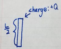
Since the electric field produced by a charge at any given location is proportional to the distance from the charge to that location, we will need to relate the observation location to the source of the charge, which we will consider the origin of the rod. To do that, we will need to divide the rod into pieces of length \delta y each containing a charge \delta Q. In the image below, you can see what this looks like and the relation that can be found between the observation location and the source, forming the distance vector \vect{r}.
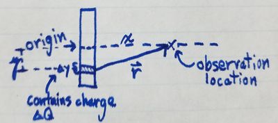
By the pythagorean theorem, we can find the vector \vect{r} as follows:

And to find the unit vector in the direction of \vect{r}, \hat{r}, we do as
follows:
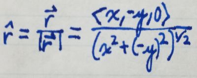
Finding the Contribution of Each Piece to the Electric Field
Now that we've set up a model for the system, with the rod broken down into pieces, we can find the contribution of each piece to the electric field of the system. We will start from the electric field equation you learned for a point particle but plug in the parameters for the rod system into the equation.
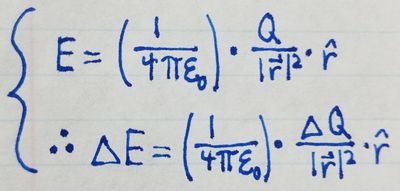
By mathematically simplifying, we then get the following equation:

Finding the Net Contribution of all Pieces
In the previous section, we found out the contribution to the electric field at a given location of only one of the pieces constituting the rod. In order to figure out the net field at any particular location, we need to add up the electric fields produced by individual pieces along the length of the rod.
We will switch from vector notation for the electric field to the scalar notation for the x- and y-components. (From the vector in the equation above, we can see that the z-component of the electric field at any point is always 0.) The x-component of the electric field is the sum of the x-components of every \delta{y} along the rod, and the y-component of the electric field is the sum of the y-components of every \delta{y} along the rod. We can show this mathematically:
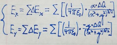
To make use of this relation, because we don't know \delta{Q}, we need to
relate it to parameters that we already know about the rod system we're
analyzing. We can express \delta{Q} as the charge density of the rod
(which is Q/L) times the \delta{y} we've chosen for the system. Thus,

By plugging the above equation into our equations for the x- and
y-components of the electric field at a point, we can find the electric
field at any point in the system. This technique is called numerical
integration and is typically done by computers because the computational
complexity is dependant upon the size of \delta{y} with respect to L.
Simplifying
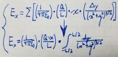
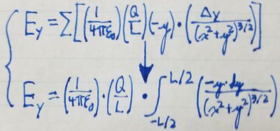
Using calculus, we can simplify a lot of the math required to compute the electric field at any given point. Notationally, all we're doing is switching from the discretely-sized \delta{y} to \textit{dy} and from the sigma notation to an integral starting from -L/2 (the lower end of the rod) and ending at L/2 (the upper end of the rod) as follows:
By evaluating the integral, we can determine that the x-component of the
electric field at any point is:

Without evaluating the integral for the y-component of the electric field,
we can use symmetry to determine that the y-component of the electric
field at any given point is 0. Let's consider the contributions to the
electric field from the top and bottom halves of the rod at any
observation point.
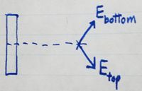
Since the y-components of E_top and E_bottom are of equal magnitude and
opposite direction, they cancel each other out, and therefore the
y-component of teh electric field at any given point due to the rod is 0.
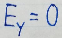
Finally, because the rod is round and can be rotated, as a convenience,
we'll use d (distance from the rod) as opposed to x (distance along the
x-direction) to refer to the electric field.
Thus we can simplify electric field calculations for a rod into a form that we can readily use:

Further Simplification
By noting the contributions of each variable to the equation for the electric field, we can make approximations to simplify our math by simply declaring one variable as insignificant.
For example, if we have a system in which the length of a rod is much greater than the magnitude of the distance from the rod (denoted L>>d), we can neglect some of the instances in which d is taken into account as follows:

Finding the Electric Field from a Rod with Code
Here is some code that you can run which shows the electric field vector at a given distance from the rod along its length. The rod is shown as a series of green balls to help emphasize that when using the numerical integrations mentioned on this page, you are measuring the field produced by discrete parts of the rod being analyzed.
Notice the edge-effects of the electric field of the rod. For reasons discussed above, if we used the long rod approximation (L>>d), these effects would be negligible.
Week 5
Potential energy
Written by Lukas Yoder, PHYS 2212 Class of Fall 2018
The Main Idea
Potential energy is the energy that an object has because of its characteristics relative to other objects within the universe. In Physics 1